CSE473/573
Fall 2010 Lecture Charts
Chapter 2: The
digitized image and its
properties
Note: You are not responsible
for Section 2.1 of 2nd Edition.
Sampling
Given a
continuous image fc(x,y),0<=x<=X, 0<=y<=Y,
we can define
sampling intervals Δx and Δy and
create a sampled image fs(j,k), which
is a matrix
whose values are
uniformly spaced samples from fc:
fs(j,k)=
fc(jΔx,kΔy), j=1,...,X/Δx, k=1,...,Y/Δy
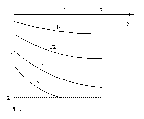
Eg: fc(x,y)= x2/(y+1),
0<=x<=2, 0<=y<=2.

For Δx= Δy = 1/2, the sampled image is the
4x4 matrix fs(j,k) where
fs(j,k)
=
fc(j/2,k/2) =
fc(.5,.5) fc(.5,1) fc(.5,1.5) fc(.5,2)
fc(1,.5) fc(1,1) fc(1,1.5) fc(1,2)
fc(1.5,.5) fc(1.5,1) fc(1.5,1.5) fc(1.5,2)
fc(2,.5) fc(2,1) fc(2,1.5) fc(2,2)
=
1/6
1/8
1/10
1/12
2/3
1/2
2/5
1/3
3/2
9/8
9/10
3/4
8/3
2
8/5
4/3
CSE573 Fa2010 Peter Scott 02-02
Using this sampling formula, the value of
each
sample (pixel) is the value of the the
continuous
image at the lower right-hand corner of
its grid cell.
If you prefer, you can sample at the
upper left-hand
corner of each grid cell by sampling
according to
fs
(j,k)=
fc
((j-1)Δx,(k-1)Δy),j=1,...,X/Δx, k=1,...,Y/Δy
or the value in the
center
of the grid cell:
fs
(j,k)=
fc
((j-.5)Δx,(k-.5)Δy),j=1,...,X/Δx, k=1,...,Y/Δy
Real devices such
as CCD cameras in fact are none of
the above "ideal
point
samplers", but store the average
brightness over
each grid cell:

CSE573 Fa2010 Peter Scott
02-03
How many samples are
needed?
Def: The bandwidth
B
of a one-dimensional signal f(x),
0<=x<=X, is the highest frequency
component needed to
expand f(x) as a sum of sinusoids
f(x) = a0+a1sin(2πFx+θ1)+a2sin(4πFx+θ2)+
...+ansin(2nπFx+θn)
Here F=1/X is the fundamental
frequency of
f(x)and
the term with frequency 2kπF is called the kth
harmonic component
of f(x).
Eg:

The greater the bandwidth, the more terms
required
in the Fourier expansion of the signal.
Rapid variations
anywhere in f(x) are indicative of high
bandwidth.
CSE573 Fa2010 Peter Scott 02-04
Shannon sampling
theorem: Let the continuous image
fc(x,y) have bandwidths U and V
in the x and y directions
respectively. Then fc(x,y) can
be perfectly reconstructed
from its samples fc(jΔx,kΔy) if
Δx <1/2U and Δy < 1/2V.
In other words, if there are more than two
samples per
period of the highest frequency component
in f(x,y),
we have lost no information in representing
it
by its
sample set.
The quantities 2U and 2V are referred to as
the Nyquist
sampling rates
for f(x,y). They are the minimum density
of samples per unit distance in the x and y
directions
to satisfy the Shannon sampling theorem,
i.e. recover
the orginal continuous signal fc(x,y)
perfectly from its
sample values.
The Nyquist sampling rates correspond to
two samples
per period.
CSE573 Fa2010 Peter Scott 02-05
Eg: If we know an image has bandwidth
20 cycles/mm
in
both x and y directions, then we need
greater than 40
samples/mm in order to be able to
reconstruct the image
from its samples with zero loss of
information.
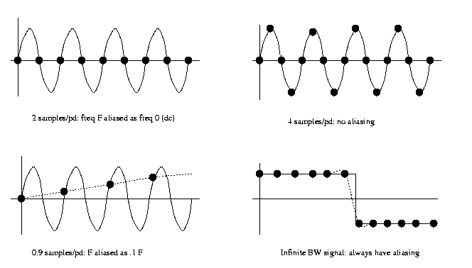
If Δx >= 1/2U or Δy >= 1/2V, the
sampling theorem is not
satisfied. The samples are too widely
spaced. In this
case we cannot
reconstruct the signal fc(x,y) from its
samples without
error.The
errors produced in the effort
to reconstruct the
continuous signal from its samples are
called aliasing errors.
CSE573 Fa2010 Peter Scott 02-06
Eg aliasing errors:

Aliasing errors are what you see with the
"wagonwheel"
or other strobe effects. These are due to
inadequate
sampling in time rather than space, but the
principle
is the same.
When you zoom in one a stripe or
checkerboard pattern
with a digital camera you see sudden jumps
in the
apparent pattern period. That's aliasing
too.
CSE573 Fa2010 Peter Scott 02-07
Quantization
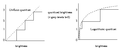
The mapping of continuous image intensity
into a set of
2b values. This permits each pixel (picture element,
picture cell) to be stored in b bits.
Typical values are
b=1 (binary image), b=8 (256 grey levels or
colors),
b=24 ("true-color" images, 224=16,777,216
colors).
The quanta can be uniform or
logarithmically scaled,
the latter reflecting the human brightness
sensitivity
curve.

CSE573 Fa2010 Peter Scott 02-08
Binary images are very useful in defining logical
image
properties, for instance, set inclusion. A
binary image
would be used to define the set of edge
pixels of an
image or the set of pixels belonging to a
given object.
8 bits are sufficient for most intensity
(graylevel)
images, as the human eye cannot
discriminate many more
levels nor can most display devices
accurately display
them. 8 bits can also define 256 colors in
an indexed
image.
24 bits are reserved for true-color
images, 8 bits
per primary color.
CSE573 Fa2010 Peter Scott 02-09
Color Models
A color model consists
of a specification of three
numbers to represent
a given color. Just as many
different sets of 3
basis vectors can be used to
lay out 3D-space, so
there are many different color
models. Some of
the models use three primary colors,
others use properties
such as intensity and saturation.
Here are some
important examples of color models, others
are mentioned in the
text.
CSE573 Fa2010 Peter Scott 02-09a
RGB:
Every visible color
can be represented as a weighted
sum of the three
primary colors red, green, blue (RGB).
Thus by detecting the
RGB
brightness of each pixel as
a triple (r,g,b) and
quantizing each separately we can
achieve color
rendition.
Eg: (255,0,0) is
saturated red; (150,150,50) is pastel
yellow,(25,25,25) is dark grey.
CMY:
Some image devices
operate by subtraction rather than
addition of
colors (filters,pigments). The CMY system
(Cyan, Magenta,
Yellow) works on this basis.
Eg: W-Y=B, M-B=R.
CSE573 Fa2010 Peter Scott 02-10
YIQ:
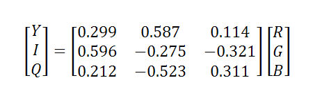
A linear transformation of the RGB model.
The Y component
is sufficient for graylevel rendition.
HSI:
Components of this model are Hue: the
dominant wavelength
in the color, Saturation: the relative
strength of the
non-white component vs. the white,
Intensity:
brightness.

CSE573 Fa2010 Peter Scott 02-10
Each of the color models can be converted
to any one of
the others. For instance, to convert RGB to
YIQ use the
linear equations

The RGB components in these equations may
be normalized or
unnormalized, yielding corresponding normalized or
unnormalized YIQ values.
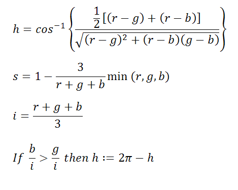
To convert RGB to HSI, first make sure the
RGB components
are normalized to [0,1], which we write as
(r,g,b). The
following formulas are then used (Edition 2
p. 26):

The s and i
components computed as above are already in
normalized form.
To normalize h take the result as
computed above
and divide by 2π. Note the angle unit in
the formula for h
is radians, not degrees.
CSE573 Fa2010 Peter Scott 02-11
Image topology and
pixel set connectedness
A blob is a set
of pixels. A fundamental image
image property is the
number
and shapes of its blobs.
A set of pixels is connected if they are
adjacent.
Blobs are usually,
but not always, connected sets of
pixels.
There are two common
ways to define adjacency :
4-neighbor: pixels touch vert or horiz;
8-neighbor: pixels touch vert or horiz or diag.
CSE573 Fa2010 Peter Scott 02-12
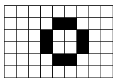
The digital connectivity paradox
In the real plane R2 of two continuous variables,
a
continuous closed curve is a connected set that
separates two other
connected sets: interior and
exterior. Not so easy
in digital plane.

Using 4-neighbor, the
interior
and exterior are
separated
(non-adjacent) but the boundary is not a
connected set. Using
8-neighbor,the boundary is
connected, but the
interior and exterior are also.
So in the discrete
plane we cannot define a boundary
simply as a connected
set separating the inside from
the outside as we can
in the real plane.
CSE573 Fa2010 Peter Scott 02-13
To chamfer
an image is to determine the distance
from each pixel to to a given blob.
Distance can
be measured by various norms:
City block
: min number of horiz/vert steps between
Chessboard
: min number of horiz/vert/diag steps
Euclidean
: straight-line length between centers.
Eg: distance between pixels
(1,2) and (5,3):
City block distance
(L1): |5-1|+|3-2| = 5
Chessboard
distance (L-infinity): max(|5-1|,|3-2|) = 4
Euclidean distance (L2):
sqrt((5-1)2+(3-2)2) = sqrt(17)
CSE573 Fa2010 Peter Scott 02-14
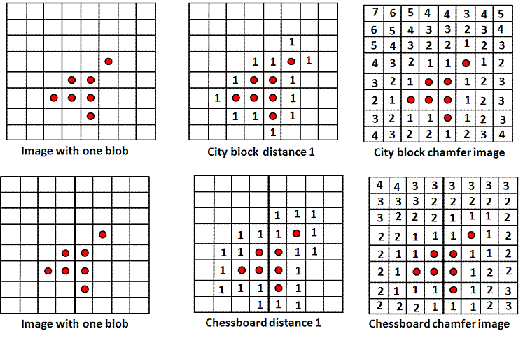
Eg: Consider the blob whose pixels are marked with a circle.
The City block chamfer
and Chessboard chamfer images are
shown.

CSE573 Fa2010 Peter Scott 02-14a
Chamfer algorithm
The chamfer image can be determined
recursively: mark the blob
pixels 0, leave other pixels unmarked. Mark
all the pixels which
are distance-1 from 0 pixels with a 1, then
mark with a 2 all
pixels that are distance-1 from pixels
marked with a 1, etc.
There is a faster way, that does not require n passes for an
image with maximum distance n. The chamfer
image can in fact
be computed in just two passes as described
on p. 28 (p. 20 of
3rd edition). Here are the steps.
CSE573 Fa2010 Peter Scott 02-14b
1. Border the image with an extra row above
and below, an extra
column left and right.
2. For each pixel p, initialize F(p)=0 if p ε blob,
else
F(p)=
∞.
3. For each p in original image, compute
F(p)=
min q ε AL
[F(p), D(p,q)+F(q)]
where D is the distance between p and q. Compute the pixels
in
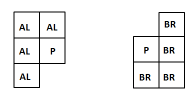
column 1 first (top to bottom), then column 2, etc. AL is
the set of 4 pixels shown
below.

4. Repeat step 3 but using BR in the
opposite order. Compute
the pixels in the rightmost column first (bottom to top)
then
move left one column, etc.
Please
note that the same correction should be made in the text
description
of Algorithm 2.1 (p 28 in ed. 2, p 21 in ed. 3).
CSE573 Fa2010 Peter Scott 02-14c
A histogram
is a count of the number of pixels at
each image graylevel from darkest to
brightest. In
the case of color images, there are three
histograms,
one for each color model component.
Eg: 4x4 3-bit
monochrome image
6
7
3
0
2
6
1
0
4
6
1
0
6
6
6
0
Histogram
h(i),
i=0,...,7:
[
4
2
1
1
1
0 6 1 ]
CSE573 Fa2010 Peter Scott 02-15
