are ready to tackle the basic issue before us,

image understanding.
 

    What objects are in the image?

    What is the meaning (semantics) of the image?
 

An image is just an array of pixel brightness values,

these numbers do not reveal themselves as comprising

parts of objects, objects or relationships between

objects without a lot of work on our part.

The first step in the process of image understanding

is segmentation, the assocation of a segment label

with each pixel. Let P={(i,j), j=1..NR,i=1..NC}

denote the pixel locations. Then segmentation is

a mapping S:P->L, where L is a segment label set.

Usually L is taken to be the non-negative integers.
 

Eg:

 0 0 0 0 0 0 1 0 0        0 0 0 0 0 0 0 0 0
 0 7 8 7 6 8 0 0 1        0 1 1 1 1 1 0 0 0
 0 7 7 8 7 8 0 0 0        0 1 1 1 1 1 0 0 0
 0 6 8 9 8 7 1 0 0        0 1 1 1 1 1 0 0 0
 0 7 7 7 6 7 0 0 0        0 1 1 1 1 1 0 0 0
 0 0 1 0 0 0 1 0 0        0 0 0 0 0 0 0 0 0
 1 0 1 0 0 0 0 0 0        0 0 0 0 0 0 0 0 0
 0 0 0 0 1 9 8 9 9        0 0 0 0 0 2 2 2 2
 0 0 0 0 0 0 8 8 8        0 0 0 0 0 0 2 2 2

  Original Image           Segmented image

                          0: background segment
                          1,2: foreground segmentS

The segmented image as above is also called the label

image.

The goal of segmentation is to group together pixels

which are similar in some important way, and

distinguish groups of pixels which are different.

Then using the size, shape, and other characteristics

of these segments we may be able to build objects out

of the segments and match these objects with known

objects, making sense out of the image.
 

Threshold-based segmentation
 

The simplest sort of segmentation is into two segments,

called the object segment (or foreground segment)and the

background segment, by comparing each pixel value to a

fixed threshold T.

Eg:

   Original image       Threshold-segmented label image
 

It is important to set the threshold T properly. If you

do not have domain knowledge specifying T, consider

the histogram of the image. If the object and background

brightness values tend to cluster in two compact sets,

the histogram will be bimodal (two main peaks) and the

threshold can be set in the valley between the modes.
 

Eg:

In choosing the valley of the histogram, we are modeling

the histogram as the sum of a foreground and a background

histogram. The pixel classification errors are those to

the left of the valley that are truly foreground pixels

plus those to the right that are background.

Eg: For a given image the threshold is selected at the

arrow.

    The pixels that will be misclassified are shown in

    red. Note they are a small fraction of all pixels.

A more rigorous approach is to find the threshold that

minimizes the probability of misclassification under the

assumption that the image consists of a sum of two

populations of pixels which are statistically defined:

foreground pixels with greylevel distribution which is

Gaussian with mean m₁ and standard deviation s₁, and

background with mean m₂ and s.d. s₂. This amounts to

fitting the histogram with a "Gaussian Mixture" 

model then finding out where the two curves cross.
 

The area under the tail of the leftmost Gaussian

to the right of the threshold is Pr(error 1).

That under the tail of the rightmost Gaussian to

the left of the threshold is Pr(error 2). To

minimize the sum, put threshold where they cross.

To see that this is the best threshold, note that

if we use a threshold which is set a little to left

of the curve crossing we are adding more error 1

than subtracting error 2. Same applies on the other

side of the crossing, adding a bit more error2 than

we are reducing error 1.
 

Due to uneven lighting, a good threshold in one

part of the image may not be good in another. Thus

can subdivide the image and do separate thresholding

in each subimage.
 

Regions where it is difficult to find a good threshold

(no valley, not bimodal), thresholds from neighboring

regions can be interpolated.
 

Multiresolution threshold segmentation
 

Multiresolution image processing algorithms operate

on several copies of the same image at different

resolutions (eg. image pyramids formed by 2x2 avg).

Top-down algorithms make a coarse estimate of

something near the top of the pyramid then refine it

as they descend down. Bottom-up or data-driven

algorithms compute values at small scales, then

combine the values by averaging or refinement as

they ascend up.
 

Multiresolution threshold segmentation works by

computing a threshold at a coarse level near the

top, then refining it by recomputing it in the

border region between segments on the next lower

level.

Threshold-based segmentation has limited usefulness.

Often, many of the pixel values within an object are

the same as in the background or another object. For

instance, a person might be weall a blue shirt and

be imaged against a blue wall. The regions need to be

distinguished by shape rather than raw pixel values.
 
 

Edge-based segmentation methods
 

The idea here is to define the boundaries of segments

using edge detectors. The segment is then defined as

consisting of all the pixels inside the bounding edge.

Or there may be multiple interior segments within one

larger one.
 

Recall that edge detection is a differentiation-based

operation, and that always increases noise. Thus

a major issue in edge-based segmentation is how to

"clean up" the set of edges so that they are simple

connected sets with an inside and an outside. There

are three major problems to be addressed:
 

    1. Edge thinning

    2. Edge connecting

    3. Elimination of isolated small fragments
 
 

 
Thinning: One approach is to use morphology

 operators to be discussed later. Another is

 to estimate the edge direction, then for each

 candidate edge pixel:

    1. Examine other candidate edge pixels

       across edge profile (perpendicular to

       edge direction).

    2. Mark the maximum valued pixel as an edge

       pixel and the others not.
 

    Eg: Use a compass operator (eg. Prewitt, Sobel)

    to get an edge image plus edge direction (N, NE,

    etc.) at each pixel. Threshold to identify strong

    candidate edge pixels. Then for each candidate

    edge pixel, take max of it and its two connected

    neighbors in direction of the maximum directional

    derivative, mark that one an edge pixel others not.
 
 

 
Connecting: Single pixel breaks in edges can

 be corrected by examining a 3x3 window centered

 at each non-edge pixel. If there are unconnected

 edge pixels in the window, mark the center an

 edge pixel.
 

    Eg:   0 1 0 0 0 0 0 0 0 0    0 1 0 0 0 0 0 0 0 0
          0 0 1 0 0 0 0 0 0 0    0 0 1 0 0 0 0 0 0 0
          0 0 1 0 0 0 0 0 0 0    0 0 1 0 0 0 0 0 0 0
          0 0 1 1 0 0 0 1 1 1    0 0 1 1 0 0 0 1 1 1
          0 0 0 0 0 0 1 0 0 0    0 0 0 1 0 0 1 0 0 0
          0 0 0 0 1 1 0 0 0 0    0 0 0 0 1 1 0 0 0 0
          0 0 0 0 0 0 0 0 0 0    0 0 0 0 0 0 0 0 0 0
          0 0 0 0 0 0 0 0 0 0    0 0 0 0 0 0 0 0 0 0
          0 0 0 0 0 0 0 0 0 0    0 0 0 0 0 0 0 0 0 0
 

 A related approach is to use dual thresholds,

 a method called threshold hysteresis. Mark all

 pixels with edge value > T1 as edge pixels, then

 all pixels > T0 (a lower threshold) if they are

 connected to a marked edge pixel. Recall that this

 2-threshold strategy was also used in the Canny edge

 operator.
 

Elimination of isolated small edge fragments:
 

Thresholding of the edge image will remove the

weaker fragments due to noise. A bigger problem

is real edges but on a smaller scale than we

are interested in.
 

Eg:
 
 

     From CityHall.jpg     After Sobel Filter
 

One approach is to run an edge connector, then

zero out all edge fragments smaller than a

certain size.
 

CSE573 Fa2010 Peter Scott 05-14

---

 

Edge relaxation
 

Basic idea is to iterate on confidences of the

edge locations. As confidences go to 1 or 0, we

have an emergent edge map.
 

The edge locations most often used are called crack

edges, ie. edges between two 4-connected pixels.

A given crack edge has a vertex at each end.

There are four kinds of vertices: 0, 1, 2 and 3.

The label corresponds to the number of other crack

edges meeting our given crack edge at that vertex.
 

CSE573 Fa2010 Peter Scott 05-15

---

Eg:
Crack edge (3,4)-(3,5) has upper vertex of type

0 and lower vertex of type 1. Left vertex of

(1,6)-(2,6) is of type 2 while right vertex of

(2,1)-(3,1) is of type 3.
 

A type n-m crack edge is one such that one vertex

is of type n and the other of type m. In the

example, the crack edge (2,2)-(3,2) is a type 1-3.
 
 

CSE573 Fa2010 Peter Scott 05-16

---

 
    Iteration goes as follows. Initialize all confidences

of all crack edges in the entire images to values

between 0 and 1 based on available domain analysis,

preliminary processing or edge filter. Then for each

crack edge, alter its confidence according to its

type. Reinforce 1-1 crack edges the most, penalize

0-m crack edges the most. When you are done with all

crack edges, that terminates a single iteration of

the relaxation algorithm. Repeat. Continue until

relaxation coverges to 0 or 1 for all crack edges. That

is, the maximum absolute difference of any crack edge

from either 0 or 1 < threshold, max_i(min(|c_i-0|,|c_i-1|)<T.

 

CSE573 Fa2010 Peter Scott 05-16a

---

 

How do you decide the type of a vertex when you only

have confidences for the adjacent 3 crack edges rather

than sure knowledge of the neighboring crack edges?

There are formulas (5.13, p. 141) for deciding this

based on the three confidences. Basic idea is that if

you have, for instance, high confidence that two of the

three neighbors on one end have type 1 vertices and the

other you are confident is a type 0, you would increase

your confidence your crack edge has a type 0 vertex there

and decrease your confidence in the other types at this

vertex. Further details and extensions are discussed in

the text.
 
 

CSE573 Fa2010 Peter Scott 05-17

---

 

Border tracing
 

Edge based segmentation uses edges to define and/or

encode segments. Suppose we have labelled a segment,

assumed to be a connected blob. Finding its border

permits chain coding or other segment border coding

schemes to be applied.
 

Inner boundaries are connected sets of pixels which

are within the blob but are each adjacent to at

least one pixel outside the blob. Outer boundaries

are connected sets of pixels not in the blob, but

are each adjacent to at least one pixel in the blob.

Either can be used to characterize the border.
 
 

CSE573 Fa2010 Peter Scott 05-18

---

 
 

Eg:

    Eg: 1-connected outer boundary pixels shown with

    o's. Note that if you use 4-connectivity to define

    adjacency between a candidate pixel and the interior

    of the blob, you end up with an 8-connected boundary,

    and vice versa. All six blob pixels are inner boundary

    pixels.
 
 
 

CSE573 Fa2010 Peter Scott 05-19

---

 

Ideally, adjacent segments should share a common

border. With either inner or outer boundary borders,

this does not happen.
 

Extended border: roughly, shift the inner boundary

one-half pixel outward (details p 144-5 text).
 

Eg (continued):

CSE573 Fa2010 Peter Scott 05-20

---

 

Graph search methods for border finding
 
 

Suppose we have the edge strength s(x) and the edge

direction Φ(x) for each pixel x = [i;j] in an

image. We can construct a directed attributed graph

in which the nodes are the pixels (attributed with

its edge strength). The arcs, representing candidate

border transitions, are entered according to a set

of graph connection rules. For instance, add an arc

from x_n to x_m iff:
 

   I. They are 8-connected;

  II. The gradient in x_n points at x_m plus/minus 45

       degrees;

 III. s(x_n) and s(x_m) are both > T_s, a strength

      threshold.
 
 

CSE573 Fa2010 Peter Scott 05-21

---

 

Eg:

Now suppose we are seeking the best border between

pixels x_i and x_j. Define a cost function associated

with any path in the graph connecting x_i and x_j. The

problem becomes one of searching the graph for the

path of minimum cost beginning with x_i and ending with

x_j.
 

CSE573 Fa2010 Peter Scott 05-22

---

 

One method to search the graph is by exhaustive

enumeration. For each non-looping path connecting

the begin and end nodes, compute the cost and

select the optimal one.
 

For cost functions which are the sum of individual

positive node costs such as this, several powerful

algorithms can be used to reduce the computation time.

One is to use the A*-algorithm. This algorithm is

of the "shortest-path" class, and is widely used

in games and simulations as well as image processing.

CSE573 Fa2010 Peter Scott 05-22a

---

Call n_A the start node and n_B the end node.

Define the path cost at any node ni as the

sum of the cost from n_A to n_i plus an estimate

of the cost from n_i to n_B. Note: in estimate = 0,

this is referred to (as in the text) as the A-algorithm.
 

    0. Let n_i=n_A and the the OPEN list be empty.

    1. Expand n_i and add its thusfar unvisited

       successors to the OPEN list with pointers

       back to n_i.

    2. Find the OPEN node n_i of minimum overall

       path cost, remove it from the open list.

       Terminate successfully if n_i=n_B. Terminate

       unsuccessfully if OPEN list is empty. Else

       go back to step 1.
 
 

CSE573 Fa2010 Peter Scott 05-23

---

 

There is a step-by-step numerical example in the

text on p. 150 (Fig. 5.22). The numbers in a node

are the estimated costs from that node to the end

of the problem. See text for details.
 

 

  Main aspects of Fig. 5.22 (see text for full figure)

The estimates used have a critical effect on the

properties of the algorithm. If the estimate of

the cost from n_i to n_B is zero (A-algorithm), it will

terminate in the optimal, minimum-cost path. Otherwise,

the algorithm may run much faster, but optimality is

not guaranteed.
 

The node costs may be taken to be constant (minimum

node-length path) or "inverse edge strength"
 

     node cost at x_i = (max_images(x)) - s(x_i)
 
 

CSE573 Fa2010 Peter Scott 05-24

---

Other node cost choices include border curvature,

distance from estimated border, distance from end

pixel.
 

There are various strategies for trying to keep

the size of the OPEN list small, including pruning,

branch-and-bound, and other heuristics. Multi-

resolution graph seaching can be very useful: get

an approximate solution at low-res, then kill all

nodes at high-res except those near the low-res

solution.
 
 

CSE573 Fa2010 Peter Scott 05-25

---

 

Border finding by Dynamic Programming
 

Suppose we have a monotonic and separable cost

function we are trying to minimize in traversing a

graph. Richard Bellman's Optimality Principle

observes that any portion of an optimal path is

itself optimal. In other words, if an optimal path

goes through n_i and n_j, then the portion of the

path between n_i and n_j is the optimal path (minimum

cost path) which connects these two nodes.
 

Applying this idea recursively to the terminal

portion of the optimal trajectory, we can construct

an algorithm which reduces the problem of N-step

optimization to many one-step optimizations. This

results in a dramatic computational reduction.
 
 

CSE573 Fa2010 Peter Scott 05-26

---

 

Eg: Find the optimal path which starts at node 2 and

    ends at either node 15 or 16. The branch costs

    (cost of moving between the nodes connected by

    the arrow) are shown.

 

CSE573 Fa2010 Peter Scott 05-27

---

 
 

The cost-to-go function V(n) for any node n measures

the minimum cost path beginning at n and ending at

one of the goal states. If there is no such path,

mark the cost-to-go from n as infinity (or "x").
 

The Bellman Equation being used throughout states

that the cost-to-go from n equals the minimum sum

of branch cost from n to m plus cost-to-go from m,

minimized over all nodes m that can be reached in

one step from node n.
 

The branch costs in the Dynamic Programming algorithm

can be set to the node costs at the destination nodes

of the arrows, in which case the algorithm finds the

minimum sum of node costs solution. Other costs that

can be selected may include a node cost plus a cost

proportional to the difference in gradients between

the nodes, length of path between nodes, etc.
 
 

CSE573 Fa2010 Peter Scott 05-28

---

 

Note: the DP search can also be done in the forward

direction as described in the book. The backward DP

search as described above is usually preferred, as

it leads to a border map which tells us for each

possible start state, the optimal border from there.

Eg (continued):

 

CSE573 Fa2010 Peter Scott 05-29

---

 

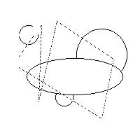
Hough Transform
 

If the size and shape of desired segments are known

in advance, but their location is unknown and their

edge boundaries in the image may be noisy or

partially occluded, the Hough Transform is a useful

tool for locating them.
 

Eg: Find all circles of unit radius and all

    broken straight lines in this image.

CSE573 Fa2010 Peter Scott 05-30

---

 
 

The Hough Transform was originally developed to find

straight lines in images. To find lines, we create

a parameter space image associated with the image

space image (input image).
 

Each straight line y = kx + q is characterized by

two parameters: the slope k and intercept q. Thus

each line in (x,y) space maps to, in other words

is in 1:1 correspondence with, a point (k,q) in

parameter space. So finding lines in (x,y) space

corresponds to finding points in (k,q) space.

 

CSE573 Fa2010 Peter Scott 05-31

---

 
 

Now each point (x_o,y_o) in (x,y) space might be part

of many possible lines, those satisfying y_o=kx_o+q

for all possible (k,q). In parameter space, this

describes the straight line q= -x_ok+y_o. So points

in image space map into lines in parameter space.

These lines "pile up" at points in parameter space

corresponding to straight lines in the digital image we

are working with.

So to find lines in image space, we will map each image

point into a line in parameter space and see where

the accumulated value is high.
 
 

CSE573 Fa2010 Peter Scott 05-32

---

 

Hough Transform Algorithm for finding straight lines:

given a discete binary image,
 

    1. Discretize parameter space into N_KxN_Q cells

       called an accumulator array. Initialize each

       cell in the accumulator array to zero.

    2. For each foreground pixel in image space

       determine the cells in the accumulator array

       that the corresponding (k,q) line passes

       through, and increment each of them by +1.

    3. The peaks in the resulting accumulator array

       correspond to detected lines in the original

       image.
 
 

CSE573 Fa2010 Peter Scott 05-33

---

 

The slope-intercept parameterization of straight

lines has the bad property of not being able to

represent vertical lines. A better parameterization

is s-theta, where s is the distance from the origin

to the line and theta the angle of the line.
 

The formula for a straight line in image space in

terms of s-theta is
 

        s = x cos(theta) + y sin(theta)
 

In this case each foreground pixel (x_o,y_o) in image space

maps into a sinusoidal curve
 

        s = sqrt(x_o^2+y_o^2) cos(theta - arctan(y_o/x_o))
 

in (s,theta) parameter space. Line-finding is done

using an (s,theta) accumulator array as described

above.
 
 

CSE573 Fa2010 Peter Scott 05-34

---

    Generalized Hough Transform  

    Any segment shape can be parameterized and found

    using the Hough Transform the same way as lines.
 

    Eg: Find all squares of side length 4 pixels which

        are aligned with the coordinate axes
.

        Let's parameterize the square by (x_ulc,y_ulc),

        the coordinates of its upper left hand corner.

        So for a given foreground pixel p in the input

        image, we will increment by one each cell in

        an accumulator array that might correspond to

        the ulc of a 4-square that p is part of.

    Region-based segmentation
 

    The third general approach to segmentation (counting

    threshold-based and edge-based as the first two) is

    to define as distinct segments sets of connected

    pixels whose properties are sufficiently similar

    to one another, and sufficiently dissimilar from

    neighboll segments. This is region-based segment-

    ation.
 

    Formally, let {Ri, i=1...S} be a candidate

    segmentation of an image and H:R->{true,false}

    where R is any subset of pixels from the image

    and H(R) true means R is sufficiently homogeneous

    relative to some underlying homogeneity criterion

    test. Then {Ri, i=1...S} is a successful segment-

    ation if H(Ri)=TRUE and H(Ri U Rj)=FALSE for

    every i=1..S and (i,j) adjacent.
 
 

    The similarity metric or homogeneity criterion

    might be based on color, gray level, rate of

    change of gray level, or some other scalar function

    which determines how similar two pixels are.
 

    The order in which new pixels are recruited into

    existing segments, or new segments started, has

    much to do with segmentation performance. The main

    ideas here are split, merge, and watershed

    segmentation.
 

    Merge segmentation
 

    Idea is to start with very small candidate segments

    (regions) and merge them together. Typically, the

    initial regions are single pixels or very small

    groupings.
 

        1. Define an initial region set {R_i} and a

           homogeneity test H based on a homogeneity

           measure (e.g. gray level similarity).
 

        2. For i=1..S_k, for j=1..S_k adjacent to R_i,

           if H(R_i U R_j) is true, merge R_i and R_j.
 

        3. Iterate step 2 until H(R_i U R_j) is false

           for all adjacent regions.
 
 

    Several possible H's for merge segmentation are

    discussed in the text.
 

    Eg: Let h(R) be the histogram for region R. Define

        the homogeneity measure
 

            S(R) = mean(h(R))/sd(h(R))
 

        where mean and sd (standard deviation) are

        computed considering the histogram h() as a

        prob density fn. Then H(R)=TRUE iff S(R)>T.
 

    Eg: Let S(R) = W/min(per_i,per_j), where W is the

        count of weak crack edges between regions i

        and j (|x(n_i,m_i)-x(n_j,m_j)|<T_w for crack edge

        (n_i,m_i)-(n_j,m_j)) and per_k is the perimeter

        of region k. Then H is true iff S(R)<T.
 
 

    Merge segmentation, being pure bottom-up, tends

    to suffer from "tunnel vision," it is not aware

    of the surrounding regions and their properties.

    Thus you tend to get a lot of small regions in

    the end, or if the threshold is low, merging of

    distinct regions together.
 

    Idea is to start with very large regions, then

    split them if they do not satisfy the homogeneity

    test.
 

        1. Build an image pyramid based on 4:1 avg.

           Let level 0 be the top level, level n the

           bottom (full resolution) level. Let k=0.
 
 

        2. Examine each cell R_i not marked CLOSED on

           level k. If H(R_i)=TRUE, mark R_i as a distinct

           segment and mark all descendent cells of R_i

           CLOSED.
 

        3. Repeat 2. for k=0,..,n-1.
 

        4. Label all not-CLOSED cells on level n as

           distinct segments.
 

        Eg: Homogeneity test: H=TRUE if maximum gray level

        difference between children is <4. 4x8 pixel

        4 bit gray level image.
 

        Level 0:             9   12
 

        Level 1:          12 11 11 12
                          04 09 12 13

        Since children of 12-cell on level 0 pass the

        H-test, mark that region as segment 1 and mark

        all its descendant cells closed.
 

        Level 0:            9    R1
 

        Level 1:          12 11 CL CL
                          04 09 CL CL
 

        Level 2:    12 11 05 10 CL CL CL CL
                    13 12 04 09 CL CL CL CL
                    04 04 04 09 CL CL CL CL
                    04 04 09 14 CL CL CL CL

        Two of the four Level 1 cells pass the H-test.
 

        Level 1:          R2 11 CL CL
                          R3 09 CL CL

        Level 2:    CL CL R4  R5  CL CL CL CL
                    CL CL R6  R7  CL CL CL CL
                    CL CL R8  R9  CL CL CL CL
                    CL CL R10 R11 CL CL CL CL
 

        So we end up with 11 regions, largest being 16

        pixels and the smallest 1 pixel big.
 
 

    An obvious defect with split segmentation is that

    adjacent regions on different pyramid levels can

    be identical but will appear as distinct segments.

    An algorithm that combines the advantages of both

    split and merge region building is the split-merge.
 

        1. Preconditions: a homogeneity test H, initial

           segmentation and a standard 4:1 image pyramid.
 

        2. For each current region R if H(R)=FALSE split

           into 4, if H(R')=TRUE where R' is the union

           of the four children of one parent merge them,

           if H(Ri U Rj)=TRUE for adjacent regions merge

           them.
 

        3. Repeat step 2. until no further split-merges.
 

     Variations to basic split-merge are discussed in

     the text (split-link, single-pass split-merge).
 
 
 

    segmentation called watershed segmentation.

    A watershed ridge is a connected segment of local

    maxima orthogonal to the ridge direction, ie.

    one-dimensional profiles across the ridge all

    exhibit local maxima there.
 

    Watershed ridges divide catchment basins, regions

    with downhill paths to a common local minimum in

    the region (the catchment drain). Each catchment

    basin constitutes a segment in watershed segment-

    ation.
 

    in current use work from the catchment drains up,

    using a flooding operation to identify and fill

    catchment basins. Let b_min be the darkest gray

    level in the image. All b_min pixels are identified

    and assigned segment numbers. Connected neighbors

    are merged. Then b_min+1 pixels are similarly

    assigned. Watershed are identified as "dams"

    separating segments.
 

    Matching
 

    A final method of segmentation for known object

    shapes is matching. A template (matched filter)

    of the object is constructed and positioned at

    location (u,v) in the image. A match criterion

    C(u,v) is computed for each (u,v) in the image and

    the local maxima of C(u,v) are thresholded to

    determine the matched segments.
 

    Eg: Find cross patterns 0 1 0 . Image is 4x10:
                            1 1 1
                            0 1 0
 

    0 0 1 0 1 1 0 1 0 1
    1 0 1 1 0 1 0 0 0 1
    0 1 1 0 1 1 1 0 0 0
    1 0 0 0 0 1 0 0 0 0
 

    Lets use C(u,v)=1/(#differences+1), where (u,v)
    is the ULHC of the template location. Then the
    C(u,v) image is

    1/5 1/3 1/8 1/4 1/6 1/7...
    1/3 1/6 1/4 1/7   1 1/6...
    ...

    Note: you are not responsible for Section 5.5 in 2nd ed

    (6.5 in 3rd ed).