After we have segmented out of an image one or more

blobs of interest, we need to move away from

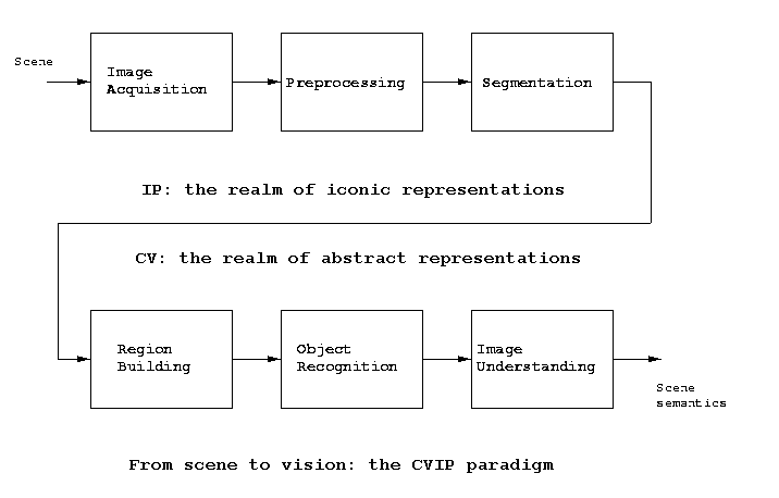
image processing towards computer vision. Recall this

block diagram:

Morphology operations, because they are image-to-image

operations, are in the image processing domain. The schemes

for shape representation and description of this chapter

initiates our look at the computer vision domain

characterized by abstract, non-iconic representations and

by increasing reliance on domain knowledge as we try to

discover image semantics.
 

There are two general approaches to shape representation:

contour-based and region-based. But as a preliminary step,

we often must first identify the distinct blobs created by

the previous step of segmentation. This is called region

identification or region labelling.
 

Region identification
 

The goal is to label each pixel belonging to a distinct

blob by a common integer identifier, and all other pixels

populating other blobs by other integers. Here is a simple

two-pass region identification algorithm for binary images:
 

  1. Set n=0, start with an empty label image and an

     empty equivalence table.

  2. Traverse the binary input image in a raster scan

     fashion.

     For each foreground pixel encountered, mark that pixel

     in the label image with the label of any of its

     neighbors.

        (a) If the neighbor labels disagree, see if there is

            an entry in the equivalence table containing any

            of these labels. If so, add all current neighbor

            labels to this entry. If not, make an new entry

            in the equivalence table containing all current

            neighbor labels.

        (b) If no neighbor is labelled, increment n and

            label that pixel by the value n.
 

   3. For each entry in the equivalence table, select one

      label and relabel all pixels belonging to this

      equivalence class with this label.

    Eg: Using 4-connectivity,

    Eg: Same example using 8-connectivity:

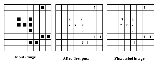
    The equivalence table has two entries: {2,3} and {4,5}.
 
 

Region labelling can be just as easily achieved from a run

length coded image or a quadtree representation. Once we

have extracted a region, we are now ready to move on to

shape description.
 

Contour-based representations and descriptors
 

Chain code: this is a representation that was discussed

earlier in context of boundary detection. The basic one

is called Freeman's chain code, which we detailed in Ch 3

(see lecture slide 03-03).variations are the

    Radial Chord Distribution: given the border of a blob B,

    define a chord for B as any straight line segment that

    has both its endpoints on border pixels of B. Let R(B) be

    the set of all chords for B. Then the histogram of R(B) with

    respect to the chord length r, designated  h_r(r), is called

    the radial chord distribution of B. This geometric descriptor

    is rotationally and translationally invariant. It also scales

    as the size of B scales, ie. the shape of the hr(r) is

    affine-invariant (invariant under any affine transformation).

    Eg:

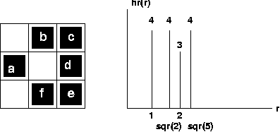
    Perimeter, area, compactness: these can be easily

    derived from chain code or other region representations.

    Area is just the number of pixels in the region,

    perimeter the number of entries in the chain code, and 
 

            Compactness = 4*pi*Area/Perimeter²
 

    These scalar descriptors are very coarse, telling little

    about the detailed shape of a blob, so are useful mainly for

    clustering and screening. Clustering is identifying sets of

    regions which share similar characteristics, and screening is

    detecting regions which have some coarsely specified

    characteristics to determine candidates for a more

    refined search or classification procedure.
 

    Eg:  We wish to count asbestos fibers in an image

    containing them in a matrix of more compact mineral

    grains. We segment the image, label the blobs,

    measure the compactness of each blob. Find a

    cluster with compactness < 0.1, visually sample

    the clusters and find these to be mostly asbestos,

    other clusters to be mineral grains. Then screen

    for further measurements by compactness threshold.
 

    in a segment S of the set of boundary pixels. The

    curvature of S, c(S) = card(C(S))/card(S). Curvature

    pixels are pixels where the boundary changes

    direction significantly, and can be defined in a

    variety of ways.
 

    Eg: Let P={p₁...p_m} be the ordered interior boundary

    of a region (p_i+1 adjacent to p_i, p₁ adjacent to p_m).

    Define pi as a curvature pixel iff the angle formed

    by {p_i-n, p_i, p_i+n} <= theta.

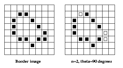
and chord distribution, see text p. 239. You are not

responsible for Fourier Descriptors, p. 240-241.
 

Sequence representations of boundaries
 

The chain code boundary representation is based on

the idea of characterizing each one-pixel boundary

segment. This can be generalized by approximating

multi-pixel boundary segments. The approximators

can be straight lines, curves from some class, or

even a class of lingusitic terms called primitives.

A primitive is a geometric label we apply to a segment

of the boundary we are describing.
 

Eg:

  Primitives: a = straight segment

              b = shallow cw curve segment

              c = sharp cw curve segment

              d = shallow ccw curve segment

              e = sharp ccw curve segment

  Syntactic description in terms of the primitives

  starting from top: bacacecabbab.
 

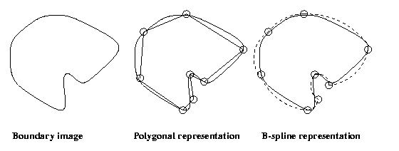
Each method has its advantages: polygonal approximations

are simple, characterized by the vertices only. Spline

and other explicit curve representations are more complex,

characterized by vertices and curve parameters, but more

accurate. Syntactic descriptions are robust, size and

angle invariant, intuitive, but least accurate.
 

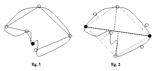
    Polygonal approximation: how many vertices and where

    should they be located? The more vertices the better

    the approximation. For a given number of vertices,

    they should be optimally selected to minimize the

    mean square error. Effective algorithms typically only

    approximate the optimal vertex locations.
 

    Eg 1: Pick the boundary pixel of highest curvature

    as the start pixel. Add pixels to the first segment

    as long as the ms segment error < tolerance. Use the

    first pixel that fails as the next vertex.
 
 

    Eg 2: Find the two pixels of maximum chord length.

    For each half-boundary separately, find the pixel

    of maximum deviation from linearity, use that as

    a vertex. Recursively select new vertices until

    desired number of vertices or tolerance is met.

  Scale-space boundary representations
 

A problem with most boundary representations is that

a given curve looks different at different scales (res-

olutions). This makes matching error-prone.
 

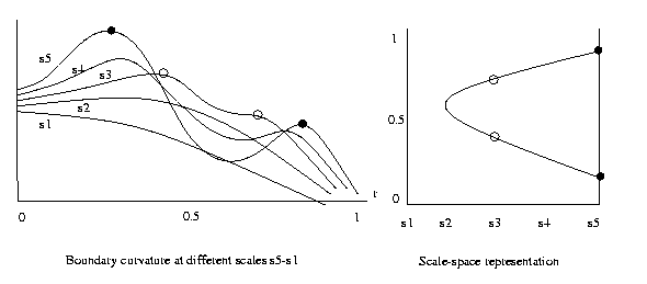
A scale-space image v(s) is a scale-invariant represent-

ation of a boundary or any other curve. To get v(s):
 

    1. Compute a curvature function C(r) of the boundary

       using the full resolution available. C(r) approx-

       imates the rate change of the slope; 0≤ r≤1 is a

       location parameter along the boundary.
 

    2. Compute the Laplacian-of-Gaussian of C(r) using

       variance s. Peaks are the points of max curvature

       in the boundary at resolution s.
 

    3. Plot the locations of these peaks vs s. This is

       the scale-space image of the boundary.
 

Eg:

    C(r)                                                                                   v(s)

B-spline boundary representations
 

Consider a portion of a boundary shown in the ULHC

figure in the next slide, 6-15, with the selected

vertices for a segmental representation indicated.

Assuming our boundary representation will pass through

the vertices, how are we to interpolate inbetween?
 

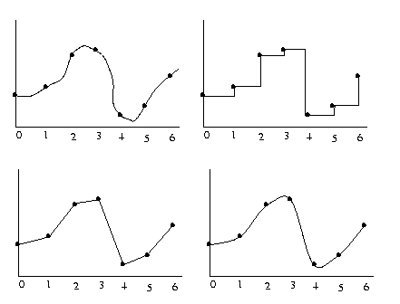
B-splines of order 1 represent constant interpolants,

order 2 piecewise-linear interpolants, order 3

piece-wise quadratic interpolants, etc. Here are the

shapes of the basis functions:

So the first basis function for order-1 b-splines is

φ ₁₁(x)= 1 for 0≤ x≤1, and φ ₁₁(x)= 0 otherwise. Order 2

b-splines have two linear segments, order 3 have three

quadratic segments, etc.

Interpolation by B-splines of order n has some nice

properties:

    1. Zero interpolation error at vertices ("knots").

    2. All derivatives up to order n-2 are continuous

       everywhere, even across knots.

    3. Interpolation is local, if a knot value is

       changed the interpolant only changes over an

       interval of length n.

    4. Interpolation is just a linear combination of

       identical, shifted basis functions.

Eg: 1D function, order 1, 2, and 3 B-spline approx.

Note: do not worry about the formulas for B-spline

      work given in Sec. 6.2.5. They apply only to

      to special case (n=4, piecewise-cubic).
 

Boundary representation by invariants
 

A scalar property of a geometric object (eg. boundary

curve) is said to be invariant under a specified group

of invertible transformations if the value of the

property is not changed by the transformation.
 

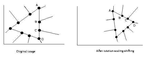
Eg: The angle formed by 2 lines is invariant under

    shifts, rotation and scaling transformations

    (affine transformations).
 

Eg: A straight line connecting two points is still

    a straight line after a perspective transformation.
 

An approach to representing boundaries is to find an

invariant description. Then, when the object is present

in a transformed image, it can still be recognized.

Cross-ratio: Mark four ordered points A, B, C, D on a

straight line. The cross-ratio I=((A-C)(B-D))/((A-D)(B-C))

is invariant under affine transformations. In this formula,

(A-C) is the Euclidean length of the segment from pixel A

to pixel C, etc.

Eg:

 
Recall from our discussion of Hough transform that four

lines that intersect at a single point map into four

colinear points in slope-intercept parameter space:

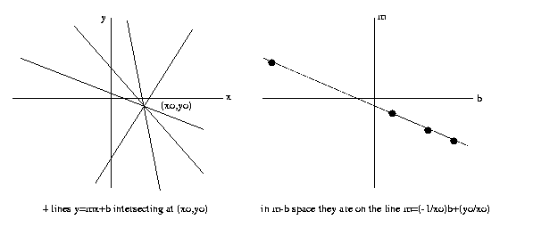
Since the cross-ratio of the four points in invariant,

so would be the cross-ratio of the four lines they

parameterize. This is one use of the cross-ratio invariant.
 

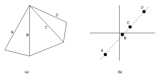
Eg: In an image, we have a figure with a corner shown

in (a). Then we can map the four lines into m-b space

as in (b), compute the cross-ratio. For any affine

transformation, we would look for a corner composed

of four lines, map into m-b space, check the cross-

ratio. If it is the same object, it will be the same

cross-ratio for both.

 

A set of any five coplanar points has two invariants,

see (6.26) p 251 for details.
 

Another class of geometric objects for which there are

known invariants is the class of conics (conic sections),

that is, planar curves that can be represented as
 

            ax²+bxy+cy²+dx+ey+f=0
 

or in vector notation as the quadratic form
 

                x^TCx=0

where   C=[a b/2 d/2; b/2 c e/2; d/2 e/2 f]

and     x=[x;y;1]'.
 

A pair of conic sections has two affine-invariants

I₁ and I₂, where

    I₁={Tr[C₁^-1C₂]|C₁|}/{Tr[C₂^-1C₁]²|C₂|
 

and I₂ is I₁ but with its indices 1,2 reversed.

Eg:

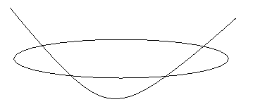
C₁=[1 0 0; 0 2 0; 0 0 1]; C₂=[1 0 0; 0 0 1; 0 1 0]

|C₁|=2, |C₂|=-1, C₁^-1=[1 0 0; 0 1/2 0; 0 0 1],

C₂^-1=[1 0 0; 0 0 1; 0 1 0],

C₁^-1C₂=[1 0 0; 0 0 1/2; 0 0 1]; Tr[C₁^-1C₂]=2

C₂^-1C₁=[1 0 0; 0 0 1; 0 2 0]; Tr[C₂^-1C₁]=1
 
 

Additional invariants for a single conic section

together with a pair of lines or points are given

in (6.29).
 

Region-based representations and descriptors
 

As with segmentation, shape representation can be

approached via boundary or region-based methods.

One problem with most boundary-based methods is

that they are sensitive to noise and to small

variations of the boundary. Region-based methods

tend to be more tolerant of noise and distortion,

ie. more robust. Also, they do not depend upon

prior boundary detection.
 

Other advantages of region-based over boundary-based

descriptor methods are ease of affine transformation

and compatibility with syntactic methods. Disadvantages

may include computational complexity and dimensionality.
 

Scalar region-based shape descriptors
 

A rough description of the shape of a blob can be

captured by specifying the values of a set of

geometric region parameters such as area, elongatedness,

horizontal and vertical projections, etc. These do not

constitute a lossless description but are adequate for

many screening and rough-matching purposes.
 

Area simply means pixel count of the binary

blob. Can be computed by region labelling

followed by counting pixels with a given

label. Can also be computed directly from

quadtree or chain code shape representations.

For quadtree, suppose the image size is 2^Hx2^H.

Then at each foreground leaf at level 0<=h<=H,
 

             area += 4^(H-h)
 

Note that any region shape description can be computed

from quadtree, chain code, or any other lossless

representation by first mapping back to the image

of the region.

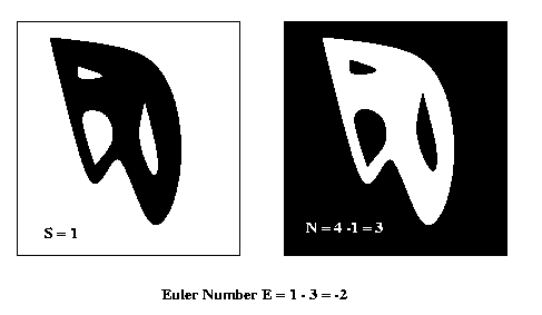
        Euler number is a useful topological property

        i.e. a property invariant under rubber-sheet

deformations)

        of binary blobs. It is defined as E=S-N where

        S is the number of connected foreground seg-

        ments in the blob and N the number of

        holes, or connected background segments within

        the blob. E can be computed by region-labelling

        the blob, then region-labelling within the blob

        after reversing foreground/background.
 

        Eg:

        Note that the Euler number does depend on whether

        4- or 8-connectivity is used to count the segments.


        Eg: consider an image consisting of a diagonal line of n

        foreground pixels. Using 8-connectivity, E=1-0=1. Using

        4-connectivity, E=n-0=n.

        Projections: the horizontal projection p_h(i)

        is, for each column i in the image of the blob,

        the count of the number of foreground pixels

        in that column. p_v(j) defined similarly.
 

        Eg: Can tell the orientation of a square from

            its projections.
 

        Eccentricity: maximum chord length divided

        by maximum perpendicular chord.
 

        Elongatedness: area divided by (2d)², where

        d is the erosion lifetime of the blob.
 

See text pages 258-259 for additional scalar region

based shape descriptors: rectangularity, direction

and compactness. Others are circularity, convex

composition number, convexity degree.
 

    Shape description by moments
 

Let f(i,j) be the image of a single binary or gray scale

blob B. For p>=0 and q >=0 define the (p,q)th moment of

B m(p,q) and the (p,q)th central moment mu(p,q) by

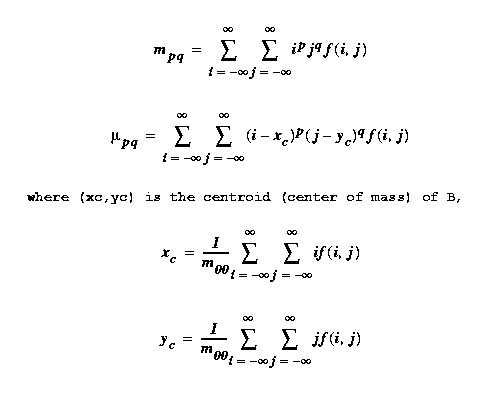
Central moments have the advantage of being translation

invariants, ie. if g(i,j)=f(i+k,j+l) for all i, j then

the moments m(p,q) of g and f will differ, but the

central moments mu(p,q) will all be the same. This is

true because the central moments are really moments about

the centroid of the blob, and when you translate the

blob by say (k,l) pixels you also translate the centroid

by the same amount.

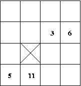
Eg: Find the (0,0) and (1,2) moments for this image:

Moments are the coefficients in an infinite power

series expansion of the Fourier Transform of f(i,j).

The Moment Representation Theorem^[1] says that f(i,j) may

be exactly reconstructed from the complete set of its

moments {m(p,q),p>=0,q>=0} or {mu(p,q),p>=0,q>=0}. In

practical applications, a finite (usually small) number of

the low-order moments are used to describe a blob.
 

^[1] Jain, Fundamentals of Digital Image Processing, Prentice Hall 1989
 

Typical use of moments is in moment matching. A finite

number of moments of an object template will be stored,

then compared to the measured moments of each blob in

an image to determine if it matches.
 

To facilitate the matching process, invariant moments

are often used. These are sets of moments which are

invariants of specified transformation groups (eg.

translation, scaling, affine). Several examples of sets

of invariant moments are given on pages 260-261.
 
 

Convex hull
 

A region is said to be convex if every pair of points

within it can be connected by a straight line that

lies entirely within the region. Regions with holes,

"fingers" or "dimples" are not convex.
 

The convex hull of a region R is the smallest convex

region containing R (intersection of all convex regions

containing R).

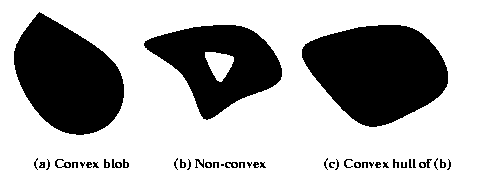
The convex hull CH(R) of a region R can be represented by

its extreme points, the set of boundary points of R which

are contained in bounding lines of R (lines that intersect

the boundary of R but not its interior). CH(R) can be

constructed by intersecting the half-spaces formed by the

set of all its extreme points.
 

Eg: Construction of the set of extreme points of CH(R).

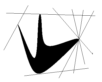
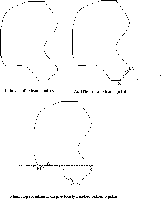
Here is one algorithm for identifying the extreme points

(and thus the convex hull) of a general region R.
 

    1. Find the pixels with the largest row index in R.

       These are extreme points of R.

    2. Likewise, the pixels with the smallest row index,

       the largest column index, and the smallest column

       index are extreme points of R.

    3. Let P1 be the pixel in 1. above with the largest

       column index. Moving ccw along the boundary one

       pixel, call this pixel P2. Form an angle whose

       vertex is P1, one arm of the angle being the line

       segment P1-P2, and the other being the horizontal

       line beginning at P1 and extending to the right.

    4. Holding P1 fixed, repeat step 2 moving ccw along the

       boundary until the first marked extreme point is reached.

       Mark the pixel P2* with the minimum such angle as the

       next extreme point.

    5. Repeat step 3 above, replacing P1←P2*, and replacing

       the horizontal line by the extension of the line segment

       connecting the previous two extreme points found. 

    6. Continue in this manner around the figure until you

       return to the original P1. 
 

Eg:

 
In Chapter 11 we saw several methods for deriving

the skeletons of blobs: maximum ball skeletons,

medial axis transform skeletons, and homotopic

skeletons by sequential thinning. These (and other)

skeletonization procedures can be used to derive

a graph which describes the shape of the blob. In

the graph, endpoints of the skeleton (points with

just one skeleton pixel neighbor) are leafs, junction

points (points with three or more neighbors) are

non-leaf nodes, and nodes are connected by arcs if

there is a direct skeleton path between them (no

intervening nodes).
 
 

Eg:

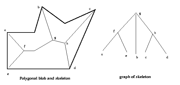
Note that the graph is invariant under a wide range of

shape transformations that preserve the structure of

the skeleton of the blob, such as affine transformations

and curvature distortions.
 

Finally, a common region-based shape representation

strategy is the decompose the object into a set of

simple pre-defined geometric objects called primitives.

The primitives and their spatial relationships are

gathered into an attributed non-directed graph in

which edges represent adjacency. This graph

is the shape description of the object.
 

This method is often used in CAD/CAM to build up

3D representations of rigid objects of complex

shapes. Given a 2D image, the model is projected

in various poses to find matches for a given blob

in an image.
 

    Eg: 2D primitives of hexagon, circle, ellipse,

        rectangle.

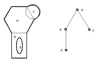
    The attributes of node H (hexagon) are its size,

    location, pose and type 'OBJECT'. R has attributes

    of major axis, minor axis, location, pose and type

    'OBJECT'. Similarly C (circle) has radius, location,

    and type 'OBJECT'. E (ellipse has major axis, minor