Some computer vision applications require no more than

the successful implementation of steps discussed so far.
 

Eg: Count the number of blobs of size >10 pixels.
 

Eg: Determine if the single object in the image (a gear

    imaged on a conveyer belt) has the correct number of

    teeth.
 

But these are only the simplest of computer vision

applications. The majority requires more than mensuration,

the quantitative measurement of scene attributes.

Typically we need to recognize or classify the objects in

the scene. This requires more than the ability to segment

and then characterize shape of each candidate object in

the scene, it also requires domain knowledge.

Questions that cannot be answered without domain knowledge:
 

    1. What kind of objects are we looking for?
 

    2. What are the defining characteristics of these

       objects?
 

    3. How may instances of these objects vary from some

       ideal instance (eg. size, pose, lighting)?
 

This procedure is referred to as object recognition (OR). It

brings together shape representations derived from the

image with data structures and algorithms which represent

object classes and methods for matching. These may be

pre-selected and unchanging, or they may be modified as

the system operates. If this modification results in

performance enchancement, this process is called learning.
 

Knowlege representation
 

Since we propose to combine domain knowledge with

generic image analysis data, we need to know how

this domain knowledge is to be represented. There

are many forms which can be used to represent

knowledge:
 

    1. Vectors of scalar parameters;

    2. Probability density and mass functions;

    3. Set of IF-THEN rules;

    4. Graphs and nets (semantic and neural;

    5. Predicate logic, fuzzy logic, other logics.
 

Specific methods of knowledge representation make most

sense within the context of the methods of object rec-

ognition that use them. So we will proceed to develop

the principles of several alternative approaches to

object recognition.

In general, there are two broad approaches to object

recognition, by analysis and by synthesis.
 

    OR by analysis: describe each candidate object by

    a vector of pre-determined features. Decide the

    class of the candidate object by mapping the

    feature vector into decision space.
 

        Eg: Nearest-neighbor classification.

        Eg: Bayes optimal classification.

        Eg: Vector quantization.

        Eg: Neural nets.
 

    OR by synthesis: describe each candidate object

    by a procedure for synthesizing that object.

    Decide the class of the object by comparing the

    synthesis procedure to stored class template

    synthesis procedures.
 

        Eg: Grammatical pattern classification.

        Eg. Classification by production rules.

        Eg. Sematic nets.

The first class of methods we will study employs analysis

based on feature vectors and probabilities. It was the

first pattern recognition method systematically devel-

oped, and probably today still the most common in

applications:
 

Statistical Pattern Recognition
 

Our goal is to correctly classify objects. Assume there

are R classes of objects {ω₁...ω_R} defined in the domain.

The statistical approach is to compute, for each possible

decision rule d() we might use,
 

    Pr( guess ω _i and true object is ω_j | use d() ).
 

We can then decide, on the basis of these probabilities,

which d is best. For instance, we might select the d

that leads to the minimum probabilility of error. Or

we may define a loss function which varies from error

to error, and select the d which results in the minimum

average loss.

Let x=[x₁ x₂ .. x_n]^T be the feature vector, and

Ω ={ω₁..ω_R} be the set of class identifiers. Let

d: Rⁿ-> Ω  be a decision rule associating with each

possible value of the feature vector x a class

identifier. Let D_k(d)={x: d(x)=ω_k} be the kth

decision region, ie. the region of feature space

that d classifies as ω_k. The set of boundary points

between the decision regions are called the decision

boundaries or the discrimination hyper-surfaces.

If each of the discrimination hyper-surfaces is linear,

the decision rule is said to be linear.

Eg:

 

One way to determine these decision region boundaries

is to define a set of discrimination functions g_i(x)

and specify that the decision region D_k(x) is the set

of points x in feature space characterized by
 

    D_k(x) = {x: g_k(x)>=g_i(x) for all i=1..r}
 

So each decision region D_k(x) is determined to be the

region of feature space X where its discrimation function

g_k(x) is the maximum discrimination function.
 

Then the question for decision function design becomes,

how do we select the discrimination functions {g_i(x)} so

that the decision rule D_k(x) they define is the one we want? 
 
 

There are two classes of procedures for computing discrim-

ination functions, and thus decision rules. One is based on

probabilities, and leads to statistical decision rules.

The other does not compute or estimate probabilities and leads

to direct decision rules. We will first look at a direct

decision rule, the minimum distance classifier.

Minimum distance classifiers
 
 

First we must define a training set. Let a single

correctly classified instance x, ie. a duple {x,ω}

with x in X and ω in {1..R} be called a training

atom, and a set of such be called the training set

for this classifier.

Then the minimum distance classifier is defined as

the classifier (decision rule d_MD(x)) that will classify an

unknown instance x as belonging to class r if and only if

the nearest training atom to x is labeled class r. The

sense of "nearest" can be chosen to be Euclidean distance,

city block distance or any other norm.

If the distance metric is selected to be Euclidean,

then the classifier turns out to be geometrically

simple to visualize. This is due to the fact that the

locus of points equidistant from any two points in Rⁿ is

the hyperplane which is perpendicular to the line segment

connecting these two points and passes through the

midpoint of that line segment.
 

Using the Euclidean norm, if there is just one training atom

per class, the decision rule is always linear.
 
 

If there are two or more than one training atoms for at

least one class, in general the decision rule is

piecewise-linear.
 
 

To determine the minimum Euclidean distance classifier

discrimination boundaries in R²,
 

    1. Construct all the perpendicular bisectors of

pairs of training atoms with different class labels.
 

    2. For each such bisector, say bisector A, mark a

point on it which is far distant from the training set.

Determine if the two atoms defining A are closer to it

than any other training atom. If so, move in towards the

training set along this bisector until it intersects

another one of the perpendicular bisectors constructed

in step 1. Mark the segment of A beginning at that point,

passing through the point where the construction began,

and going on to infinity as a discrimination segment.
 

    3. Repeat 2. for the other end of each bisector.

    4. Define a bisector segment as a segment of

a bisector which lies between intersections with two

other bisectors, and contains no other such intersections.

For each bisector segment, determine if the two atoms

defining it are the closest atoms to it. If so mark that

bisector segment as a discrimination segment. Mark all

bisector segments.

    5. The union of all discrimination segments found in

steps 2-4 above are the required discrimination boundaries.
 
 

In terms of discrimination functions for minimum distance

classification we can use the set
 

              g_i(x) = 1/G_i(x)
 

where G_i(x) is the minimum over {x_j,i} of training

data labelled class i of the distance between x and

x_j. Any other monotone increasing function of this

minimum distance can be taken as g_i(x) as well. To

keep the discriminant functions well-defined every-

where and avoid dividing by zero, the definition
 

              g_i(x) = 1/(G_i(x)+1)

is often used.
 

Minimum error classifiers
 

The problem of classifier design is to determine a

decision rule d(x) which tells us, for each x in the

feature space X, what classification we will assign

to an object which has that particular feature vector. 

As we have seen, the decision rule can be encoded in

the selection of a set of discrimination functions

{g_i(x), i=1,...,R} which tell us how to decide the class

of each x in X. For each x, d(x) will evaluate to the

label i of the largest g_i(x).

So lets assume we have an x we wish to classify. Let

P(ω_r|x) denote the probability that the true class

is r, given that feature vector x. Then for minimum

error classification, we can assign a set of discrim-

ination functions
 

            g_i(x) = P(ω_i|x)
 

So if we can compute P(ω_i|x) for each x and each ω_i,

we can use these probabilities as our discrimination

functions, and have our minimum error classifier.
 

How can we compute P(ω_i|x)? The most common way is using

Bayes Law, which says that for any two events A and B,
 

        P(A|B) = (P(B|A)P(A))/P(B)
 

Bayes Law follows from the definition of conditional

probability,
 

        P(A|B)=P(A,B)/P(B)

thus    P(A,B)=P(A|B)P(B)=P(B|A)P(A)
 

The form we will use Bayes Law here is
 

        P(ω_i|x)=(P(x|ω_i)P(ω_i))/P(x)
 

P(ω_i) is called the a priori probability of ω_i.

This is the likelihood of class i before we see the

data x. P(x|ω_i) is called the class-conditional like-

lihood of x given w_i. P(x) is called the prevalence

of x.
 

What Bayes' Law tells us is how the a priori probability

of ω_i is updated by the data x into the desired

a posteriori probability P(ω_i|x). In other words, how the

data x has influenced our judgment of the likelihood that

x comes from class  ω_i.  

Eg: Prior probabilities: P(normal)=3/4, P(sick)=1/4.

Based on a blood test, we are given a feature vector

x with P(x|normal)=1/5, P(x|sick)=4/5. Then by Bayes Law,

    P(normal|x) = (1/5)(3/4)/P(x) = 3/(20P(x))

    P(sick|x)   = (4/5)(1/4)/P(x) = 4/(20P(x))

So if we are doing minumum error classification, we

should classify this patient as sick, since

P(sick|x)>P(normal|x).
 

 Eg continued:

    P(sick|x)   = P(x|sick)P(sick)/P(x)

    P(normal|x) = P(x|normal)P(normal)/P(x)

so

    P(sick|x)/P(normal|x)= (4)(P(sick)/P(normal))
 

Thus if the prior probability of being normal is

more than 4x larger than that of being sick, we will

decide normal even though the evidence points strongly

to being sick ("likelihood ratio" P(x|sick)/P(x|normal)=4).
 
 

Gaussian minimum error classifiers
 

The most common form for the class-conditional probability

density functions (pdfs) in practice is the Gaussian, or

Normal, distribution given by

Now we showed previously that the posterior probabilities

P(ω_r|x) form a min-error set of discrimination functions
 

         g_r(x) = P(ω_r|x) = P(x|ω_r)P(ω_r)/P(x)
 

Now any other set of functions {g_r'(x), r=1..R}

which preserves the maximum (g_k'(x)>=g_i'(x) for

all i=1..R if and only if g_k(x)>=g_i(x) for all

i=1..R) will qualify as a set of discrimination

functions just as well as the g_r(x)'s above.
 

So lets multiply each gr(x), r=1..R by a common

factor P(x), the prevalence. This preserves the maximum,

so we have a new set of discrimination functions
 

        g_r'(x) = P(x|ω_r)P(ω_r)

Now let's define
 

        g_r''(x) = ln g_r'(x)
 

Since the natural log is monotone increasing, this

also preserves the maximum, and thus defines a new

set of discrimination functions. For the Gaussian case,

Now the decision hypersurfaces are x's where the

maximum two g_r(x)'s are equal. So in the Gaussian

case they are parabolas. In the special case that

the covariance matrices are all equal, the quadratic

terms can be removed from the discriminants, along

with the other common terms, leaving

We conclude that in the Gaussian case with equal

covariance matrices, we have an important simplification:

the discrimination functions, and the decision hyper-

surfaces, are linear, ie. the decision rule is linear.
 
 

 Eg: x = s + n, where for ω₁, s = [1 1]^T and for

    ω_2, s = [2,2]^T. n is Gaussian with mean [0 0]T

    and covariance matrix psi=[1 0; 0 1] (the identity

    matrix). Assume the two classes have equal priors.
 
 

    Then

        p(x|ω₁) = 1/(2pi) exp(-1/2((x₁-1)²+(x₂-1)²))

        p(x|ω₂) = 1/(2pi) exp(-1/2((x₁-2)²+(x₂-2)²))

    The discrimination hypersurface is where the two

    discrimination functions are equal,
 

       [1 1]^Tx-1/2*[1 1]^T[1 1]+ln(.5) =

             =  [2 2]^Tx-1/2*[2 2]^T[2 2]+ln(.5)

    or

               x₁+x₂-1 = 2x₁+2x₂-4
 

    which is the straight line
 

                x₂ = -x₁+3

Minimum-average-loss classifier
 

The minimum error classifier implicitly treats all

errors as equally undesirable, and all correct class-

ifications equally desirable. But in practice this is

often not the case.
 

    Eg: In a medical screening test, false negatives

        are usually more costly than false positives,

        and true positives are more valuable than true

        negatives.
 

    Eg: In a speech driven operating system,

        classification errors leading to logouts or

        system crashes are worse than those opening a

        dropdown menu.
 

Define a loss function λ:{1..R}X{1..R}->R¹ such

that λ(ω_r|ω_s) is the loss sustained if a sample is

classified as ω_r when its true class is ω_s. Suppose we

are required to classify the sample x. The minimum-

average-loss classifier, also referred to as the

Bayes-optimal classifier, is the one which classifies

x as d(x)=ω_r where ω_r minimizes the expected loss

for this value of x,
 

    d(x) = ω_r = arg min ω_i { E[λ(ω_i|ω_s,x)] }
 

In this expression the expectation is taken over ω_s

with ω_i and x fixed.

Eg: Previous example with P(ω₁)=P(ω₂)=1/2. Lets use a

    loss function λ(ω₁|ω₂)=4, λ(ω₂|ω₁)=1,

    λ(ω₁|ω₁)=λ(ω₂|ω₂)=0. Then
 

        E λ(ω₁|ω_s,x)=4*P(ω₂|x)

        E λ(ω₂|ω_s,x)=1*P(ω₁|x)
 

    So the discrimination hypersurface will be the set

    of x such that 4*P(ω₂|x)=P(ω₁|x). But, cancelling

    common factors of P(x) and 1/2, by Bayes' Law this

    is
 

            P(x|ω₁) =4*P(x|ω₂)
 

    Equating two exponentials and taking logs, this

    turns out to be a linear decision rule.
 

           ln P(x|ω₁) = ln P(x|ω₂) + ln 4

    where

      P(x|ω₁) = 1/(2pi) exp(-1/2((x₁-1)²+(x₂-1)²))

      P(x|ω₂) = 1/(2pi) exp(-1/2((x₁-2)²+(x₂-2)²))
 

        (x₁-1)²+(x₂-1)² = (x₁-2)²+(x₂-2)²-2.77

           -2x₁+1-2x₂+1 = -4x₁+4-4x₂+4-2.77

                     x₂ = -x₁+1.62

If we are not given the required probabilities
 

In order to find the minimum-error or Bayes' optimal

classifier, we need to know all the class-conditonal

pdf's {p(x|ω_i), i=1..R} and all the a priori probab-

ilities {P(ω_i), i=1..R}.
 

Sometimes we assume this information is assumed to

be known and given to us during the off-line design

stage before on-line operations. In this case we have

a complete stochastic model for the classification

problem. Complete stochastic models require two

things:
 

    1. Lots of data, or complete theoretical domain

       knowledge;

    2. The assumption that the probabilities are

       invariant during on-line operations.
 

If these conditions are not met, we must learn while

on-line (while classifying) rather than in advance

while off-line during training. Learning is the

adaptation of an algorithm or behavior in light of

actual experience.
 

Eg: In a character classifier problem, we begin with

    a priori probabilities P('a'), P('b'), etc. taken

    from a general English language database. But in

    the book we are translating, we find that the

    letters 'x', 'y', 'z' show up much more frequently;

    the letter 'e' much less frequently. We recompute

    priors according to the "hits-to-trials" ratio
 

    P(wi) = (instances of wi so far)/(all letters so far)
 

    Proceeding in this way, we are learning the correct

    priors not in general for the English language, but

    for this book.
 
 

Eg: We know that x = s + n, and we know that n is

    Gaussian, but we don't know what its mean vector

    or covariance matrix are. We use a method for

    estimating these quantities from the training

    training data seen so far.
 

Suppose we are given a set of training data {x₁..x_n}

whose true class is ω_k.
 

Estimating the mean μ_k of a Gaussian:
 

        μ_k~ = 1/n (x₁+..+x_n)
 

where μ_k~ is the estimate of μ_k after n training

data. Our estimate of the mean is just the sample mean.
 

This is not the only feasible estimate of the mean,

but it has many nice properties and is usually chosen.

It is minimum-variance unbiased, maximum likelihood,

asymptotically efficient and asymptotically normal.
 

Estimating the covariance matrix ψ_k of a Gaussian:

a Gaussian: use μ_k~ above for the mean estimate,

then replace μ_k in the covariance estimate by this

μ_k~ ; also replace 1/n by 1/(n-1).
 
 

Syntactic approach to object recognition
 

So far we have considered the statistical approach

and the min-distance approach, in which objects are

characterized by their features.
 

In the syntactic approach, we construct a description

of an object in a selected formal language. Each

object class ω₁..ω_R is characterized by a grammar,

that is, a set of alphabets and relations which

govern  what strings of symbols from the formal

language are  "legal" for objects of that class.

When we have found an object class for which the

given object description is grammatical, we declare

a match to that object class.
 

Formally, a grammar is a 4-tuple G=[V_n,V_t,P,S] where
 

    V_n is the set of non-terminal symbols;

    V_t is the set of terminal symbols (primitives);

    P is the set of production rules;

    S is the start symbol.
 

We always start with S, then choose a production

rule to replace a non-terminal (intially S) by a

terminal symbol or combination of terminals and

non-terminals. We keep going until the string

contains only terminals. That is the "word" we have

created using the grammar.
 

Eg: Consider the following code grammar which produces

    "complementary mirror codes" (CMCs):
 

    V_t = {0,1,E}

    V_n = {S,X}

    P = {S->XE, X->0X1|1X0|01|10}
 

    Then for instance if we receive the string

                    00101011E

    we find it is grammatical using the CMC grammar,

    since
 

       S->XE->0X1E->00X11E->001X011E->00101011E
 
 

Types of grammars
 

The more general the grammar the more expressive

it is; the more constrained the grammar the easier

it is to parse.
 

Let x be an element of V_t; a and b be elements of

V_n, A, B and C be grammatical strings of primitives

from V_t U V_n where the symbol U refers to set union,

and e be the empty set. Then we can distinguish four

types of grammars, from the least constrained to the

most general:
 

    Type 3: Regular grammars (finite grammars):

            Left regular: a->xb|x

            Right regular: a->bx|x
 

In other words, a regular grammar works by writing

a terminal symbol and moving to a new nonterminal

state. Type 3 grammars are represented by

finite-state automata, which makes them easy to

parse.
 

    Type 2: Context-free grammars:

            a->A
 

In other words, a non-terminal can be replaced by

any grammatical string independent of the symbols

surrounding it (independent of context).
 

    Type 1: Context-sensitive grammars:

            AbC->ABC

In other words, the non-terminal b can be replaced

by the string B but only if it is surrounded by the

specific strings A and C, ie. only in this context.
 

    Type 0: General grammars:

            unconstrained.
 
 

Regular grammars and Finite-State Automata (FSA)
 

Each regular grammar corresponds to an unique FSA.

The non-terminals are the nodes and the automata

writes a terminal along each arc. There is one

additional node, the end node (an absorbing

state), which is the only FSA node explicitly

referenced in the regular grammar.
 

Eg: 4-bit code with odd parity.

    P={S->0a|1b, a->0c|1d, b->1c|0d, c->0e|1f,

       d->1e|0f, e->1, f->0}

    Here is the corresponding FSA: 

  Often the easiest way to construct a regular grammar

from a "word problem" description, is to first construct

the FSA. The key to constructing the FSA is to note

that each node in a FSA is a different state in the

construction of the string, i.e. what you need to know

in order to finish the string grammatically from there.

The formal grammar, i.e. the 4-tuple, then follows

directly from the FSA.

Eg: Above, node a: odd parity so far, 3 more symbols to go

           node c: even parity so far, 2 more to go

           etc.

Parsing is the process of analyzing a given string to

determine if it is grammatical, and if so, what sequence

of production rules produced it. The more general the

grammar, the harder it is to parse.
 

Regular grammars can be parsed by constructing a parse

tree. If the parse tree does not have a branch that

terminates immediately after the last terminal, the

string is not grammatical.
 

Eg: Determine if the string 001101001 is grammatical in

the regular grammar represented by the FSA

Start the construction by writing the terminals vertically

down a sheet of paper. Then beginning with node S at the

top, draw an arc to each node in the FSA you may reach by

outputting the given terminal. Proceed until you reach the

end of the string, or no further arcs are possible.
 

Conclude that the string is grammatical and the

unique sequence of productions is
 

   S->0d->00f->001a->0011d->00110f->001101a->

        ->0011010c->00110100e->001101001
 

Parsing is more difficult with Type 0-2 grammars

since they cannot be represented by FSA's nor parsed

using the simple parse tree described above.

Grammatical inference is the process of inferring a

grammar from a set of examples. For any finite set

of consistent examples, there exists at least one FSA,

and hence a regular grammar, that produces this set of

examples as its language. This is why regular (Type 3)

grammars are also called finite grammars.

But while every finite language has a finite grammar,

there may be a simpler Type 0-2 grammar with many fewer

non-terminals and production rules. Training of

syntactic pattern recognition systems using grammatical

inference is an active area of current research.
 

Neural Nets
 

Neural nets have been on the scene a very long time,
perhaps a half billion years. The ability of biological
neural nets to produce intelligent behavior in animals
and man has inspired the design of artificial neural nets.
 

Biological neural nets:

Information processing in the human brain takes place in
a vast interconnection of specialized cells called neurons.

When the cell body (soma) reaches threshold potential,
an action potential is fired down the axon.
 

An action potential is a 1-2 ms reversal of polarity of
the cell membrane from negative to positive.
 

Here is an image of a group of neurons taken from the primary
hippocampal region of a rat. The specimen was stained with different dies to bring out the cell body, dendrites and axon.

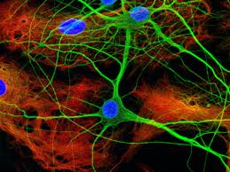
Source: nikonsmallworld.com

When the action potential reaches a synapse, or connection
with another neuron, it causes a neurotransmitter to flow
into the synaptic cleft.
 

The neurotransmitter causes the post-synaptic membrane to
become more negative (inhibitory synapse) or more positive
(excitatory synapse).

The net effect of all the post-synaptic membrane stimuli
is to change the soma potential closer to or further from
threshold.
 

In a human brain,
 

• There are 10-100 billion neurons;


• There are an average of 1-10 thousand synapses
   per neuron (10-100 trillion synapses altogether);


• Action potentials are fired asynchronously (no
   central clock signal);


• No information is conveyed in the shape of the
   action potential, only its presence or not.


• The maximum action potential rate is about 500/sec

Conclude:

• Human brain is a very large neural network.


• It operates with massive parallelism among simple
  computing elements.


• Large groups of neurons interconnected neurons have
  very similar input-output properties, but some
  differences group to group.


• The system is digital rather than analog.


• Bit coding is the rate of action potential firings.


• Information coding and memory coding unknown.


• Much slower than a pc (~ million times slower), but expoits parallelism to create speedup for some tasks (eg. face recognition) of ~ billion.

Artificial neural nets

    An artificial neural network is a highly parallel
    interconnection of simple computing elements called
    artificial neurons.

    Eg.
 
 

How do artificial neural nets work?
 

Neural nets are trained to learn a desired target function

t: X -> Y

where X is the space of input vectors and Y the output
vectors. The output y=t(x) of the neural net is the "right" output when the input to the neural net is x.

Typically the network topology (number of inputs, outputs,
neurons, and their interconnections) and the selection of
net and activation functions for each neuron, is fixed.
Learning proceeds by modifying the weights Ω = ( ω₀,..., ω_nw).

 
Consider one particular assignment of numerical values for all nw weights as a point in an nw-dimensional space. One point in this space is the true target function, its location is what we are trying to learn. The unbiased hypothesis space is R^nw. Each point in this space is a hypothesis, or guess, as to what the target function is.

    Eg. For preceeding diagram, there are (remember
        the bias inputs):

            6x4 + 5x2 + 3x3 = 43 weights

        The hypothesis space H is the 43 dimensional
        set of real numbers ω = R⁴³. Learning is moving
        from point to point in R⁴³ until a solution
        is found.
 

Learning as search over weight space
 

How do we search the unbiased hypothesis space H = Ω = R^nw?
How do we recognize a hypothesis that is better than our
current one? Start by specifying a training dataset D:

    Training dataset D: A set {(x_i,t_i)}of input
    vectors x_i and their corresponding target vectors t_i.

Let ω in R^nw represent the current weight vector. We can
assess  how well we are doing by passing x_i through the
system, noting the output o_i, and determining the
error (t_i-o_i). Then the total sum-squared error is:

 The error manifold E(ω) can be visualized as a landscape
being crawled over by an ant searching for the lowest
valley. That lowest valley is at the solution ω*, the
hypothesis in H which minimizes the error over D.
 

Gradient descent

How should we crawl over E(ω)? Gradient descent is the
approach based on finding the direction of steepest
descent, which is the negative gradient direction

Eg: Gradient descent over a 2-dimension weight space Ω
 
 

Note that gradient descent will find a nearby local
minimum, not necessarily the desired global minimum.
 
 

The Gradient Descent Rule

Let's apply gradient descent to ANN's with no hidden layers.
With E(ω) as our sum-squared error defined previously,
 
 

If we only consider the most recent error, we have
just the last term in the Gradient Descent Rule,

This is the Delta Rule. It is an incremental (rather than
batch) approximate gradient descent learning rule. It computes
the next weight vector much faster than Gradient Descent by
ignoring all but the current error. The payback is that many
more weight changes are required to convergence.
 

The Gradient Descent Rule, or its variant the Delta Rule,
can be extended to neural nets with hidden layers. A small
change in the weight ω_i will effect its neuron's outputs
and all neuron outputs downstream from it. So using the
chain rule, we can compute the partial of the  error
with respect to ω_i even for weights of hidden units.

This extension is called the backpropogation training

rule. See text page 311 for details.

    Eg.
 
 

A small change in ω₅ will cause the outputs of its neuron and all the output neurons to change, thus changing the errors at each output neuron.
 

CSE 573 Fa2010 Peter Scott 07-49

---

Eg: Classifier for a circular subset

As an example, let's use a two-input (2 input neurons), one-hidden-layer (8 hidden neurons), single-output (1 output neuron) neural net to try to learn to correctly classify points that fall inside a circular window. The target function we are trying to learn is that the neural net output should be 1.00 for input points that fall inside the circle, 0.00 for points outside the circle.
 
 

13 training atoms were used, with assigned target value of output 1.00 for the 5 points inside the circle, and 0.00 for the 8 points outside the circle.

CSE573 Fa2010 Peter Scott 07-50

---

 
The results shown below were computed using the Matlab Neural Net toolbox. It is available on all the UB machines. User guide with tutorials here.

After one epoch of training, weight training was stopped and the neural net tested.  The image below shows the result after one epoch. The output for every possible input in the range [0,1]x[0,1] is shown. Output values are coded as grey levels with pure black 0.00 and pure white 1.00. Ideally, this graph should be pure white inside the circle and pure black outside it.

The mse=0.33 (stderr=0.57) after this one epoch of training.

CSE573 Fa2010 Peter Scott 07-50a

---

After two epochs the mse is down to 0.13. It is coming closer to the desired white circle.

With additional epochs the mse decreased to about 0.09, but did not decrease further. That is because we did not have sufficient training data for the neural net to "figure out" it was supposed to be white inside a circle of radius 1/4, black outside it. With many training atoms, and many epochs, we could learn the circle with as small an error as desired.

CSE573 Fa2010 Peter Scott 07-51

---

 

Other classes of neural nets and training rules

Thus far we have discussed only feedforward
(acyclic) ANNs taught using supervised training
(input, target output training atoms).

Unsupervised neural nets learn how to cluster data in natural groupings. Instances which are (in some
sense)similar to each other are assigned to the
same cluster.

Eg:

    If the cluster at 4 o'clock corresponds to
    y2, then when the test datum comes in, the
    three outputs will be 0, 1, 0 respectively.

    An example of an unsupervised neural net is
    the Kohonen selforganzing net. Another is the
    Carpenter-Grossberg or ART net.
 
 
 

CSE573 Fa2010 Peter Scott 07-52

---

 
 

Recurrent neural nets have closed cycles in their
directed graph representations. The feedback paths
permit more complex behavior than feedforward nets.

The Hopfield net is a recurrent neural net which
operates as an associative memory. A weight matrix
Ω is formed from the set of patterns to be
remembered and y(k+1)=Ωy(k) iterated until the net
converges to a stable solution.

Eg:

For all t>2, net(t) and y(t) do not change.
Output is y(2).
 
 

CSE573 Fa2010 Peter Scott 07-53

---

Graph matching approach to object recognition
 

If the object is described by its features, then we

can use statistical methods or neural net methods for

object recognition. If it is represented as a string

of primitive symbols, syntactic methods may be used.
 

Another common method of describing objects is as

graphs. In the simplest case the nodes represent

the object parts and the arcs represent adjacency.

This results in an undirected, unevaluated graph.

    Eg:

Now if scenes (or segments of scenes) and class exemplars

are represented as graphs, object recognition amounts to

matching graphs or portions of graphs.
 

    Eg:

    Note that there are instances of this object class

    hidden in the scene.
 

Formally, a graph G(V,E) is a set of vertices V and edges

E. If the vertices are simply enumerated 1,2..N and the

the edges are designated only by the two vertices they

link without regard to order, G is called a non-evaluated,

non-directed graph. If the edges have arrows (order of

vertices in their descriptions counts) the graph is

directed, if the vertices ("nodes") or edges have

any additional attributes the graph is said to be

an evaluated ("attributed") graph.
 
 

The goal of graph matching is to find an invertible

node association function v_j'=f(v_i) between two graphs

G(V,E) and G'(V',E') such that for all k and l,
 

    1. There is an edge in E connecting v_k and v_l

       if and only if there is an edge in E' connecting

       f(v_k) and f(v_l);
 

    2. For directed graphs, there is an edge directed

       from vk to vl in E if and only if there is also

       an edge directed from f(v_k) to f(v_l) in E';
 

    3. For evaluated graphs, nodes v_k in E and f(v_k)

       in E' have identical values, also the edges

       connecting v_k and v_l in E have the same values

       as those connecting f(v_k) and f(v_l) in E'.
 

The function f is called the node association function.

In other words, for graphs to match they have to have

the same connectivity, corresponding nodes need to have

the same properties, and corresponding edges need to

have the same properties.
 

If we match an entire graph against an entire graph, this

is called a graph isomorphism. If we match a portion of

one graph against an entire other graph, this is a

sub-graph isomorphism. If we match a portion of one graph

against a portion of another, this is a double sub-graph

isomorphism.
 

    Eg: We are looking for squares in a scene. If we

        segment out a particular object from the scene

        and match it to the square graph, thats a graph

        isomorphism problem. If we match the graph of

        the square to the entire scene, we are

        seeking a sub-graph isomorphism. If we have two

        scenes both containing squares and match them

        looking for squares, that's a double sub-graph

        isomorphism problem.
 
 

      Eg:  continuing a previous example, we had the

      non-directed, non-evaluated pair of graphs

    In G, the left graph, V={1..8} and E={(1,2),(1,3),

    (1,6),(2,5),(3,5),(4,6),(4,7),(4,8),(6,7)}.
 

    In G', the other one, V'={1'..4'}, E'={(1',2'),

    (1',3'),(2',3'),(2',4')}.
 

    Consider the node assocation function f defined by

    the table
 

    In order to declare a match, we need to make sure

    that an edge exists for a pair of v's if and only

    if it exists for the same pair of f(v)'s.
 

    Check: (4,6) in E, (f(4),f(6))=(2',1')=(1',2') in E'.

           (3,6) not in E, (4',1') not in E'.

           etc.
 

    So f constitutes a valid node association function,

    and we have found a sub-graph isomorphism between

    these two graphs. 

          Note: there are 3 distinct subgraph isomorphisms

    involving G and G, not just the one we discovered

    above.

      Note that in this example, if the graphs were

      directed (arrows pointing towards the second

      node in their descriptions), then the given f

      would not constitute a legal node association

      function, since (4,6) in E is not matched by

      (f(4),f(6))=(2',1')~=(1',2') in E'.
 

      Or if node 3 had the value "blue" and node

      4' had the value "red," then f would not

      work for these evaluated graphs.
 

A useful technique for finding matches between two graphs

is based on the assignment graph. This is a matrix-shaped

graph whose rows are the nodes in G and columns the nodes

in G'. Each matrix location is a node in the assignment

graph.
 

    Eg: Nodes in the assignment graph for the previous eg.

Each pair of nodes in the assignment graph is inspected

to see if an edge should be drawn between them. The rule

is that they are connected if and only if the pair of node

associations (nodes of the assignment graph) are

consistent. Consistency requires that
 

    1. The connectivity between the two G-nodes matches

       the connectivity between the two G'-nodes,

    2. The direction of connectivity (if any) matches,

    3. The values (if any) of the corresponding nodes

       match,

    4. The values (if any) of the corresponding edges

       match.

    Only 1. is relevant for undirected unattribed

    graphs.
 

    Eg: Continued: For instance, the node association

    1 1' is consistent with 6 3' because there is an

    edge between 1 and 6, also between 1' and 3'. So

    in the assignment graph we draw an edge connecting

    nodes 1 1' and 6 3'. Also, 1 3' is not consistent

    with 3 4' because ther is an edge between 1 and 3

    but not between 3' and 4'.
 

After all legal edges are added to the assignment graph,

the matches can be readily found. A clique is a fully

connected set of nodes in a graph. Each clique in the

assignment graph specifies a legal node association

function and thus (in general) a double sub-graph

isomorphism. The maximal clique in the assignment

graph represents the largest matching set of nodes

in the two graphs. If G has n nodes and G' has m, then

a maximal clique with k matching nodes in each graph

defines a:

    1. Graph isomorphism if k=n=m;

    2. Subgraph isomorphism if k=n or k=m but not both;

    3. Otherwise a double subgraph isomorphism.
 

Example:

Start with node 11'. Consider all possible links

to nodes in second row. Since nodes 1 and 2 are

connected, add a link to each node in row 2 whose

G' node is connected to 1'. Repeat for row 3: Since

nodes 1 and 3 are connected, add a link to each node

in row 3 whose G' node is connected to 1'. Repeat

for row 4: since nodes 1 and 4 are not connected,

add a link to each node in row 4 whose G' node is

not connected to 1'. This completes node 11'.

CSE 573 Fa2010 Peter Scott 07-66

---

Repeat for each node in the association graph. Note

that links are not possible between nodes in the

same row or column. If you work from the top row

down, note that while computing the links for a given

node in a given row you need only check for links

to nodes in rows below.

The final association graph for this example is

CSE 573 Fa2010 Peter Scott 07-67

---

There are two maximal cliques (3 nodes) corresponding to two

maximal subgraph isomorphisms.

CSE 573 Fa2010 Peter Scott 07-68

---