Chapter 8: Image Understanding
Recalling the image understanding - computer vision
processing chain discussed early this semester, we
have arrived at the final step: image understanding.
Image understanding is the task of extracting complete
semantic and contextual information from a scene. This
information is usually task-dependent.
Eg:
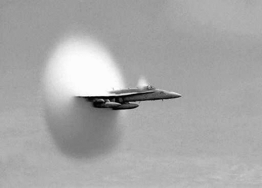
Image understanding for an air-to-air missle
would require object classification: high-per-
formance fighter, possibly detecting the national
insignia. Image understanding for a "scientifically
aware" machine vision system would require further
detecting the plume and interpreting it as signalling
that the aircraft just
broke the sound barrier.
of all significant objects in the scene, and semantic
labelling of their relationships. This scene data together
with domain knowledge is then used to derive the image
understanding.
Note: semantic labelling is labelling an object or image
part by its meaning. Eg: classifying an object, or
noting an object to be a threat. Index labelling is
labelling an object or image part by an index code
without
meaning, eg. enumerating connected segments.
Semantic labelling of objects and relationships is the
key step. The methods for doing semantic labelling include
all the methods discussed in Chapter 7: Object Recognition
plus some more: rule-based systems, semantic networks,
reinforcement learning systems, etc. In this chapter we
will survey some of these methods as applied to image
understanding.
Both image data and domain knowledge tend to be large
and weakly structured databases. So the control strategies,
that is, the order in which datasets from these databases
are selected, referenced and accessed, is very important
to the usefulness of an image understanding
scheme.
Parallel and serial control schemes: often, tasks
can be performed in parallel. If the right hardware
is available to take advantage of parallelization,
efficiency can be improved.
Eg: Divide scene into regions of interest, seach
each
ROI
in
parallel for interesting objects.
Sometimes the algorithm is inherently serial,
however.
Eg: Find the likeliest candidate to match a
desired object. Accept or, if reject, move to the
next most likely.
Bottom-up control is a sequence of transformations
beginning with the original image data, at each step
using more compact representations of image attributes
until desired semantics can be recognized. This
corresponds to a natural process of summarizing data
on multiple levels.
Eg: Pixels -> connected segments -> image regions
-> objects -> object arrangements -> understanding.
Bottom-up control is said to be data-driven, since the
decision trees are governed by the image data itself.
Bottom-up control moves up through levels of increasing
coarseness (decreasing resolution) until matching metrics
can be applied and the scene understood.
beginning with the most highly summarized image
representations available, and descending through
representations containing increasing image detail.
At each step, image structures are matched against a
library of model-based template structures of the same
coarseness (level of resolution) to determine likely
candidates for further descent and
investigation.
At each stage of descent, sub-goals are set and
executed. Top-down control is goal oriented.
image. Bottom-up, we perform edge enhancement
on the original image, then edge thinning and
connection, then find all linear features of
a minimum length, then connect them with angle
constraints, etc. Top-down, we take a low-res
version of the image, find all linear features,
search each one of those at increasing resolution
to
verify/falsify the road hypothesis.
Top-down control is model-based (model-driven). Decisions
are governed at every stage by the model attributes we
are interested in finding in the image. In the case of
bottom-up, data-driven algorithms, domain knowledge
becomes significant only in the final stages.
Other control strategies include hybrids
incorporating
both bottom-up and top-down stages (see for instance
the coronary artery border detection algorithm on p. 371),
and non-heirarchal approaches such the blackboard control
scheme. The blackboard is an open message-passing center
in which task results can be written and read, and
autonomous agents called daemons can communicate. For
instance, there can be an edge-enhancing daemon and a
segmentation daemon, along with daemons whose job is
tor identify the existence of specific states or objects
in the scene.
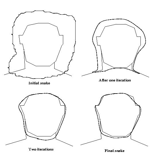
One class of model-driven control strategies is based
on active contour models, models of bounding contours
of regions whose shapes can be incrementally adjusted to
fit the image data. Active contour models which adjust
their shape consistent with minimizing a "shape energy"
functional are called snakes.
Eg: Snake model for the outline of a face. Let the
shape energy be the sum of a term penalizing the snake
for regions of sharp bending, and a term rewarding the
snake for moving to pixels of high gradient.
convergence to a local minimum would proceed in steps
such as these:
but often consists of a sum of terms reflecting three
kinds of considerations:
1. Internal energy: we typically prefer smoother,
straighter snakes to those with kinks, sharp
curvatures, and jump discontinuities.
2. Image forces: we may want to reward snakes that
tend to move to bright areas (dark areas),
that tend to track image edges, or move to
terminations (end pixels of lines or regions).
3. Constraint forces: require the snake to not be
longer than a certain legth, not enclose more
than a certain area, not be nearer a given image
feature
than a certain distance, etc.
For instance, if we wished the snake to be no more than
lo in length, we could have a term
of the form
max
(
0,
[l(s)-lo]3 )
as a constraint force. So any snake with length > lo
will be sharply penalized.
Let v(s)=[x(s),y(s)] be a point along a snake, for
s=[0,1]. s=0 corresponds to an arbitrary
starting point
along the snake, and a complete circuit of
the snake
is
made as s ranges from 0 to 1, v(0)=v(1).
Expressing the energy functional as an integral,
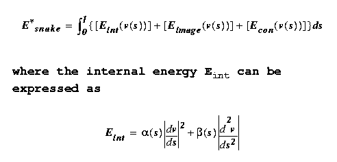
movement of the parameter s along the snake and is
called the elasticity term. The second penalizes sharp
bends or high curvature, and is the stiffness term.
The image force Eimage can take many task dependent forms.
A common generic form is to express it as a linear comb-
ination of line, edge and termination terms
Eimage = wlineEline
+ wedgeEedge +wtermEterm
If we wish to attract the snake to existing edges, for
instance, we can use the specific form
Eedge
= -| grad f(x(s),y(s)) |2
Forms for the other terms are given in the text on p376.
Using the calculus of variations, a necessary condition
for the minimal energy snake can be derived called the
Euler-Lagrange condition. This is a partial differential
equation which can be solved iteratively using standard
PDE methods.
Alternatively, the first variation (denoted dEsnake*), of
Esnake* with respect to specific variations dv(s) of the
function v(s), can be computed using standard variational
arguments. dEsnake* tells us how much Esnake* will change
if we make a small change dv(s) in v(s). The first
variation is the function-space equivalent of the first
derivative. Selecting that dv(s) which minimizes the
first variation dEsnake* we have a steepest descent
algorithm for snake construction.
Snake growing is an alternative procedure for finding the
best snake in the minimum-energy sense. It substitutes
many "easy" or small, well-conditioned snake problems for
a single "hard," badly-conditioned one. The
procedure is:
1. Get an initial snake.
2. Measure the energy density (integrand of Esnake*)
along the snake and eliminate areas of high density.
3. Grow the remaining segments by extending them along
their natural tangents.
4. Solve the snake problem for each extended segment.
5. Merge the snake segments.
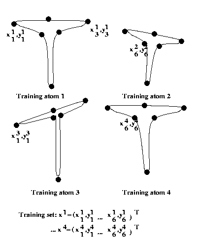
Point Distribution Models
The idea is to model an class of objects by the
locations of a set of points along its boundary,
together with the observed variations of this
pointset in a training dataset. Then when a new
instance of this object class is detected, its
set of boundary points are found by fitting to the
boundary pointset of the model (PDM). The points
in the object's PDM are connected to form the
estimate of the object boundary.
The first step in this shape description process is to
compute the PDM for the object class. The PDM consists
of two things: the vector of average locations of the
boundary points, and a set of vectors which describe
the most common variations of the boundary points from
the average, ie. the set of eigenvectors.
For each of M object images in our training dataset,
mark N "landmark" points around their boundary.
Let {(xij,yij),i=1..M,j=1..N}
be
this
set
of points.
Eg: Training set for PDM for handwritten "T"
To construct our PDM from the training dataset, first
the affine transformation that best matches xi with
x1 is found for each i. The average of the M aligned
training atoms is found, and is then aligned with x1.
Each of the aligned atoms is then realigned to match
this mean. The mean is then recomputed at the process
iterated. When converged, we have the aligned training
set {x_hat1...x_hatM}.
Computing the average of the aligned training
set
x_bar = 1/M (x_hat1+x_hat2..x_hatM)
x_bar is the expected shape of the object. But the
object class shows variations from instance to instance
which has to be
modelled as
well. Let
dxi = x_hati - x_bar
be the vector of variations or "delta" of the ith
training atom from the mean point set. Then the
2Nx2N covariance matrix of the training dataset can
be estimated as the average outer product of the
deltas,
S = 1/M ([dx1dx1]T+[dx2dx2]T+..+[dxMdxM]T)
Now S shows us the expected variation within the class.
In directions in which S is large, there is a lot of
variability in the training dataset, which in directions
of small value of S, there was little
variation.
This information is captured in the set of 2N
ordered eigenvalues and eigenvectors of the S,
S
pi = lami pi
where lam1>lam2>...lam2N are the eigenvalues and
{pi, i=1..2N} are the associated
eigenvalues.
Eg: Consider a 2-D random vector x
with mean mu
and covariance matrix S given by
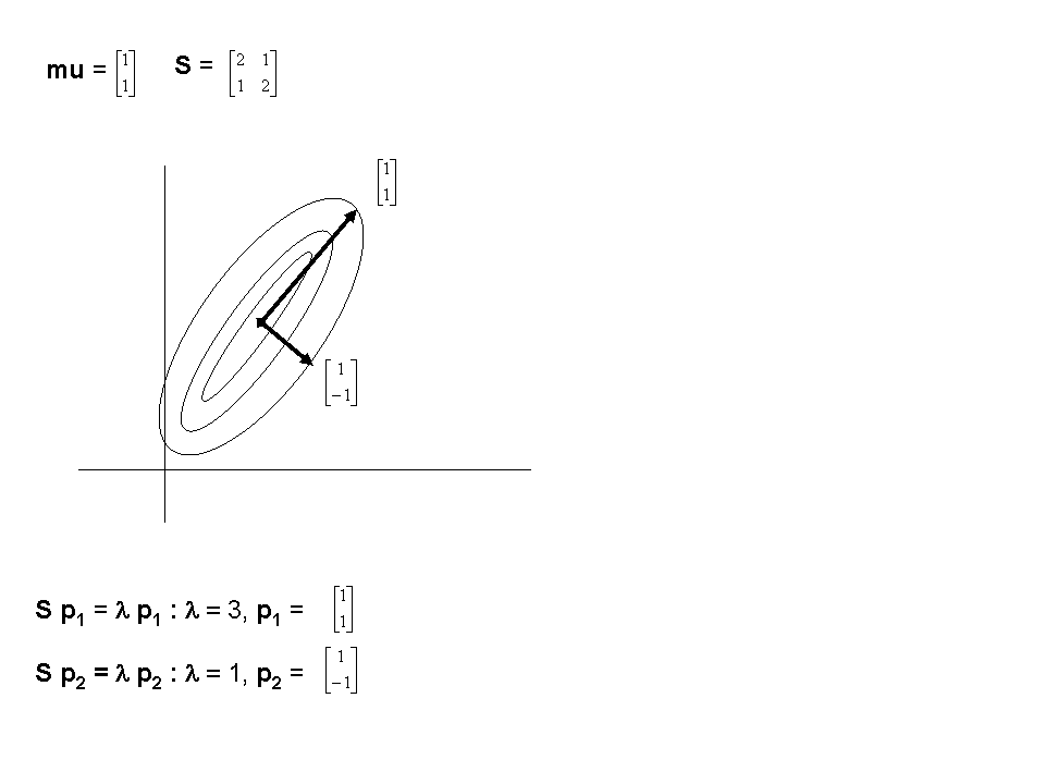
Any vector x can be represented as a linear combination
of the eigenvectors, with those corresponding to the
largest eigenvalues on average carrying the most weight.
The lower-indexed eigenvectors correspond to directions
of frequent distortion of the model class from its
mean PDM vector x_bar, the higher ones to minor
variations and noise. So the principal components
are determined by truncating the set of eigenvectors
at t<<2N and the resulting fit is
x
= x_bar
+ (b1p1+b2p2+..+btpt)
where the bi's are weight coefficients which tell how
much of each of the "modes of variation" p1..pt have
been detected in a given instance of the
object.
For details of the calculation of the bi, see
sec 8.3.
Pattern recognition
methods in image understanding
Object recognition from feature vectors was discussed in
Ch. 7. If we assign a feature vector to each pixel, the
same minimum distance and statistical techniques can be
used to answer image understanding questions
as well.
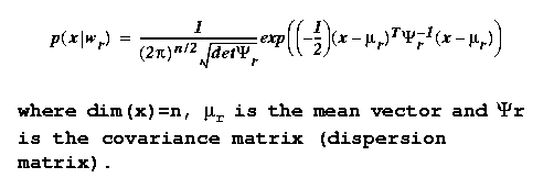
Eg: Supervised classification of multi-spectral data.
Observing the same patch of the Earth's surface
from a satellite using multiple images taken at
m different wavelengths (IR, UV, visible), let
X(i,j) be, for each pixel location (i,j), an
m-vector of brightness values. Suppose we have a
training dataset of m-vectors corresponding to
classes wheat, corn, soybeans, trees, water, grass.
Can do min distance classification of each pixel,
then postprocess with a sequence of closing
morphological operations to eliminate scattered
mislabellings.
Eg (continued): Each class of the training dataset can
be used to estimate the class-conditional
probabilities p(X|wheat), p(X|corn) etc. For
instance, for each class, we can assume Gaussian
statistics and take the sample mean as the estimated
Gaussian mean vector and the sample mean outer
product as the estimated
covariance matrix
Mu = (1/m)(X1+...+Xm)
Psi = (1/m)(X1*X1T+...+Xm*XmT)
where there are m training
atoms for this class.
The required class-conditional probabilities
p(X|wheat), etc. then take on the usual Gaussian
form
Unsupervised (clustering) techniques can also be used
on the pixel feature vectors to segment them into image
regions whose feature values are similar.
Once individual pixels are labelled, post-processing
techniques can be used to complete the image analysis.
For instance, using a rule-based system we may decide
that small regions of corn completely contained within
larger regions of soybeans should be
relabelled soybeans.
An interesting algorithm due to Kittler and Foglein uses
contextual information as the input for post-processing.
The context of a pixel is defined as the set of values of
the pixels in a neighborhood surrounding it. The basic
idea is to label a pixel by the class label wr with the
highest posterior probability given the feature vectors
of that pixel and those of all pixels in its
context.
1. Define a mask which specifies the shape and
size of the neighborhood for each pixel.
2. For each image pixel, find the context feature
vector psi by concatenating all features of all
pixels in its neighborhood.
3. Using the training dataset, estimate the class-
conditional probabilities p(psi|wr) and prior
probabilities for each wr.
4. Use Bayes' Law to determine which posterior
probability p(wr|psi) is greatest. Label the
pixel at
the origin of the mask accordingly.
Eg: Lets use a mask which biases contexts in the
horizontal direction. Mark the pixel in the mask
whose context is being defined as x0.
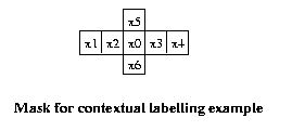
Assume in this example pixels are specified by a
scalar gray value in the range 0 to 255. Suppose
the upper left hand corner of the image is
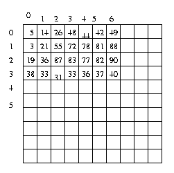
Then the context feature vector psi(1,2) is the
vector [55 3 21 72 78 26 87]T, while
psi(2,4)=[77 87 83 82 90
78 36]T
etc.
Assume there are just two classes here, w1 and w2.
We can gather all the w1 training data and compute the
sample mean mu1 and sample covariance matrix Psi1, and
assuming Gaussian statistics, we have p(psi,w1) from
the general Gaussian form (with n=7). Repeat for w2,
yielding p(psi,w2). A count of the training data in
each class gives estimates p(w1), p(w2) (eg. if there
are 100 w1 and 200 w2 training data, we estimate
p(w1)=1/3, p(w2)=2/3.
Then to label pixel (1,2), we just compare the products
p([55 3 21 72 78 26 87]T | w1) p(w1)
p([55 3 21 72 78 26 87]T | w2) p(w2)
and choose the label which agrees with the larger. To
label pixel (2,4), compare
p([77 87 83 82 90 78 36]T | w1) p(w1)
p([77 87 83 82 90 78 36]T | w2) p(w2)
Scene labelling and
constraint propogation
Image understanding is the task of extracting semantic
and contextual information from a scene. That is,
labelling objects and determining the significance
of their arrangement in
the scene.
Image understanding differs from object recognition
in that object recognition uses the properties
of individual objects to do labelling, while ignoring
context. Image understanding requires the labelling of
all objects in the
scene consistently,
that is, making
sure the labels agree
with both
properties of individual
objects and the
permissible
relationships between label
object classes.
Specified properties and relationships
are constraints on the
labels which can be applied.
A choice of object labels for the objects in a scene
that do not violate any
property or relationship
constraint is said to be consistent. Scene labelling
is the discovery of a
consistent set of
labels for
all objects in a scene.
Given:
1. Set of objects in the scene R={Ri,i=1..N}
with specified properties and relationships
2. Set of labels O={Oj,j=1..M}
3. Set of unary relations (properties) associated
with each label Pj={pj1,...,pjJ, j=1...M}
4. Set of binary or m-ary relations associated
with
pairs or m-tuples of labels,
find a consistent labelling, that is, a labelling of
each object in R such that the labels agree with all
the specified properties and relationships.
Eg: Scene with:
1. 9 objects R1..R9
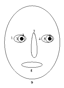
circular. R3 is in R2 is in R1; R6 is
in R5 is in R4. R8 is below R7. R7 is
between
R1
and
R4.
2. Set of labels: O1=face, O2=mouth, O3=nose,
O4=eye, O5=iris, O6=pupil.
3. Set of properties: P1={oval, square},
P2={oval, horizontal}, P3={oval, vertical},
P4={oval}, P5={circular}, P6={circular, dark}.
4. Set of relations: (Ok in O1) for k=2..6,
(O6 in O5), (O5 in O4), (O2 below O3),
(O3 on centerline of O1),
(O3 between O4 and O4).
One approach to scene labelling is discrete relaxation.
1. Assign all labels to each object which agree with
the object properties (unary relations).
2. Set i,j=1. For each object i=1,N,
a. For assigned label j, check consistency
with all relations.
b. If inconsistent with one or more, discard
that label.
c. If no labels remain, stop.
c. Repeat 2a., 2b. for all j.
3. Repeat 2. for all i.
4. Repeat 2.-3. until no further changes in label
sets for any object.
Eg (continued):
1. Check unary relations:
R1:
face|mouth|nose|eye
R2:
iris|pupil
R3:
iris|pupil
R4:
face|mouth|nose|eye
R5:
iris|pupil
R6:
iris|pupil
R7:
face|mouth|nose|eye
R8:
face|mouth|nose|eye
R9:
face|mouth|nose|eye
2. Check other relations:
R1: R2
in R1
=> face|eye
R7
between
R1
and R4 => eye
R2: R3 in
R2 => iris
R3: R3 in
R2 => pupil
R4: R5 in
R4 => face|eye
R7
between
R1
and R2 => eye
R5: R6 in
R5 => iris
R6: R6 in
R5 => pupil
R7: R7
between R1 and R2 => nose
R8: R8
below R7 => mouth
R9:
face|mouth|nose|eye
There are no empty label sets so a consistent
labelling is still possible. Repeat the check
against all non-unary relations. Find no change
so stop. We have an unique labelling of everything
except the face-object.
Need one more relation in
our knowledge base
concerning the found objects
in this image, such as
such as "R7 is in R9."
Sometimes it can take many iterations for constraints
to propogate from local label eliminations to more
distant label eliminations. For instance, if this is
not a bird then that is not a wing and then that is
not a feather may take three iterations if the bird
object is checked last, wing object next to
last.
Discrete relaxation results in consistent labelling
wherever that is possible. Sometimes, however, due to
occlusion, noise, error in computing object properites,
etc. the only consistent labelling is quite unlikely to
be correct. Sometimes we would prefer an inconsistent
but more likely labelling.
Eg: Analyzing an old photograph taken in Antarctica
in 1910. There is an object in the sky, about as
large as the sun, but with property "oval." The
discrete relaxed solution would be to label the
object as a blimp. But how likely is that? Looking
at the photo, we are more likely to interpret the
object as the sun blurred by movement of the camera
during the exposure, considering the oval property
to be an error. This would be an example of
probablistic
rather than discrete relaxation.
Probablistic relaxation
Define the support qj for a labelling ti=wk of object Ri
due to an interacting object Rj with
label tj
as
qj(ti=wk) =
sum_over_l{r(ti=wk,tj=wl) P(tj=wl)}
The total support
for ti of Ri is
Q(ti=wk) =
sum_over_j{cij*qj(ti=wk)}
where {cij} are the strength of interaction coefficients.
We iteratively relax the "probabilities"
P(ti=wk) using
P(ti=wk) <=
Q(ti=wk)*P(ti=wk)/sum_over_l{Q(ti=wl)*P(ti=wl)}
where <= is the replacement operator.
There are many variations of this basic relaxation
procedure (see text p. 462-3). They all start by setting
intial label probilities for each object in the scene
by determining image object unary and m-ary relations,
then estimating the answers to questions such
as
How likely is an iris to be square?
How likely is a UFO to
appear in this old photo?
The label probabilities are then all iteratively changed
(relaxed) using a rule such as the above. When no further
changes occur, the most likely labels for each object
are accepted, regardless of their consistency.
Finally, relaxation can be avoided by using an
interpretation tree. This is typically used in
conjunction with depth-first search with
backtracking to find a consistent labelling.
Eg: Scene has three objects, each may be an aircraft,
bird or cloud.
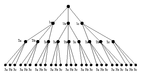
CSE 573 Fa2010 Peter Scott 08-40
Construct interpretation tree. For N objects and
M labels, tree has N+1 levels, each node has M
descendents, total of MN interpretations (leaves).
Working left to right, from root node descend to
first consistent label (no violation of unary
property for object 1). Then descend to first
consistent label from that node (no violation of
any binary property involving objects 1 and 2).
Continue until leaf reached or no consistent
label on next level. If leaf, you are done. If
no consistent label, backtrack one level and
repeat. If no new unexplored paths, declare
failure. Comment: MN
is a lot of leaves!
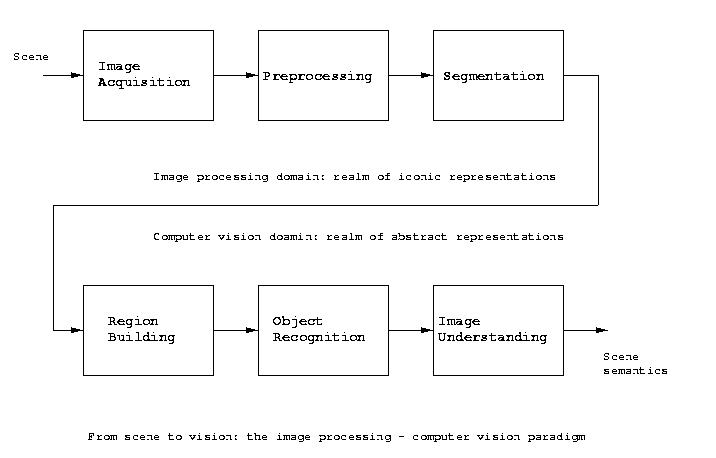
CSE473/573 Fall 2010
Summary of Topics for Final Exam
First half of the semester we worked on low-level
(image processing) steps in the image-processing -
computer vision paradigm. The second half we
concentrated on higher-level (computer vision)
steps in which the mappings were between abstract
data structures, not pixel brightness maps, and task
definitions and domain knowledge were increasingly
important.
Chapter 11, Morphology: sections 4-7 only
How can morphology be applied to analyze images?
Gray level morphology
Skeletons
Granulometry
Chapter 6: Shape reprentation and description
How do we "write down" the shape of a segment,
region or object so we can perform object
recognition?
Region labelling
Contour-based representations and descriptors
Chain code
Geometric descriptors: perimeter, area, etc.
Sequences: syntactic, polygonal, etc.
Scale space, B-splines
Invariants
Region-based representations and descriptors
Scalar descriptors: area, Euler number, etc.
Moments
Convex hull, extreme points
Skeleton graphs
Geometric primitives
Chapter 7: Object
recognition
Given the shape description of an object and a
database of domain knowledge of object classes
and their characteristics, object recognition is
the assignment of a class label to
the object.
Knowledge representation: parameter vectors,
probility fns, graphs, etc.
Object recognition by analysis
Nearest neighbor classification
Statistical pattern recognition
Decision boundaries, descrimination fns.
Bayes Law
Minimum error classification
Minimum-average-loss classification
Learning of statistical parameters
Neural nets
Artificial neurons
Learning as search over weight space
Gradient
descent,
backpropogation
Object recognition by synthesis
Syntactic (grammatical) classification
Grammars
Regular grammars and finite state auto.
Parsing regular grammars
Graph matching
(Sub-)graph isomorphisms: node assoc'n fn
The
assignment
graph:
maximal cliques
Chapter 8: Image understanding
Extract the information from the image which you
need. Recognized objects must be related and
characterized, ie. the scene contents semantically
labelled.
Control strategies
Contextual classification
Constraint propogation
Discrete relaxation
Probablistic relaxation
Interpretation tree