Morphology means "shape" or "form." Mathematical

    morphology is a set-theoretic approach to changing

    the shape of regions and segments of images. It

    is a useful basis for the design of algorithms

    for segmentation, as in Chapter 5. It is also

    widely used for preprocessing, and for object

    recognition and higher-level algorithms as well.
 
 

    Morphology for binary images   

    First we will consider only binary images. Later, we will

    extend morphology to gray level and then color images.   

    For purposes of studying mathematical morphology, we will

    represent a binary image as a point set, a subset of Z²,

    where Z² is defined as the Cartesian product of the signed

    integers, i.e. all pairs of signed integers.
 

    Elements of this point set correspond

    to the foreground (black) pixels. Each pair of

    integers defining a foreground pixel location in

    the image can be thought of as a 2D vector as well.
 

    Note: the convention in morphology is that discrete
   
    images are defined on Z², not on the Cartesian product

    of the positive integers as Matlab assumes.

    Eg: A 512x512 binary image with one black line

        running along its diagonal is the 512 member

        pixel set {(0,0)...(511,511)}. The pixel

        (10,10) can also be considered as the 2D

        column vector x = [10;10]' .
 

    Each morphological operation is a binary

    operation between the image and another point set

    called the structuring element. The structuring

    element is usually much smaller than the image

    itself, and plays a role similar to the mask

    in a small-kernel convolution.
 

    Eg: Structuring element B = {(0,0), (0,1)}.

    Eg: Stucturing element B = the 3x3 square

    {(0,0),(0,1),(0,2),(1,0),(1,1),(1,2),(2,0),(2,1)(2,2)}.
 

    Before laying out the formalities, lets

    informally look at the two most important

    morphological operations, dilation and erosion.
 
 

    Dilation
 

    Define the dilation of an image X={x} by the

    structuring element B={b} as the image Y={y}
 

    Y = X (+) B = { y=x+b for each x in X, b in B }. 

    Note: (+) in these notes corresponds to the

    operator represented by a + inside a circle

    in the text. Similarly (-), etc. to be defined

    shortly.

 

    So for each x in the image X, we color black

    all points that are of the form x+b.
 

    Eg: Consider the diagonal line image X =

        {(0,0),(1,1)..(511,511)} together with the

        structuring element B = {(0,0),(0,1)}. Then

        X (+) B = { (0,0)+(0,0), (0,0)+(0,1),
                    (1,1)+(0,0), (1,1)+(0,1),
                    (2,2)+(0,0), (2,2)+(0,1),
                    .....
            (511,511)+(0,0), (511,511)+(0,1) }

        So the dilated or "thickened" image is a

        diagonal image whose diagonal line has

        thickened from one to two pixels wide.

Note: in morphology the pixel (x,y) location corresponds

to the usual algebraic x-y coordinate orientations, not

the usual image coordinates:

      So in morphology image notation, pixel location (a,b)

      means horizontal index (col) a, vertical index (row) b.

      We will use this convention throughout our discussion

      of morphology (Ch 11 of the text).

Eg cont'd: Y = {(0,0),(0,1),(1,1),(1,2),..(511,511),(511,512)}


    For each x (col) value there are two y (row) foreground

pixels in Y, ie. we have thickened X vertically.

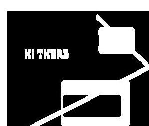
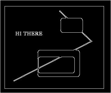
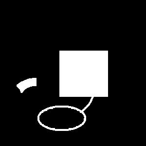
    In Matlab, use the imdilate function to produce dilation.

    Eg: >> B = ones(4);
        >> BWD = imdilate(BW,strel(B));
        >> imshow(BWD)

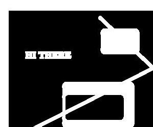
            Original Image BW                 Dilated by B
 

      Dilated by B twice         Dilated by B three times
 
 

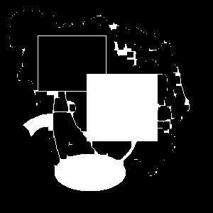
    The shape of the structuring element determines what 

    direction the image dilates, the size determines how 

    fast.

    Eg: B1={(0,0),(0,1),(0,2),..(0,7)}

        B2={(0,0),(1,1),(2,2)...(7,7)}

 
 
 

    Erosion
 

    Define the erosion of an image X={x} by the

    structuring element B={b} as the image Y={y} where
 

        Y = X (-) B

          = {y such that for every b in B, x=y+b is in X }.
 

    So for each y in Z², we check whether y+b is a foreground

    pixel in X for every b in B. If so, we color y black

    in Y. 

    Eg: X = {(1,1),(1,3),(2,3),(3,5),(3,6),(4,6),(5,7),(6,7)}

        B = {(-1,0),(0,0)}
 

        Note that since (0,0) is in B, then y+(0,0) must

        be in X in order that y be in Y, ie. if the origin

        (0,0) is in B, the only candidates for Y are those

        already in X.
 

        For (1,1) to be in Y need (1,1)+(0,0) and

        (1,1)+(-1,0) to both be in X. Not the case.

        For (1,3) to be in Y need (1,3)+(0,0) and

        (1,3)+(-1,0) to both be in X. Not the case.

 

        First one that works is (2,3), since both (2,3)

        and (1,3) are in X.
 

        Y = {(2,3),(4,6),(6,7)}
 
 

    In the previous example with B={(0,0),(-1,0)} an image

    point in X "survives" the erosion only if there is

    another image point on its left. So for instance, a

    black vertical line n columns wide erodes to n-1 cols

    after one erosion, n-2 after two, etc.  

    Note repeated: in morphology image notation, pixel location

    (a,b) means horizontal index a (col a), vertical index b

    (row b counting positive upward).

    With B={(-1,-1),(-1,0),(-1,+1),(0,-1)...(+1,+1)}, ie.

    the point (0,0) and its eight nearest neighbors, a

    point survives erosion by this B only if all of its

    eight-neighbors are in X. Thus with this structuring

    element, pixels on the boundary of a blob melt away, or

    erode away, when the erosion operation is performed.
 
 

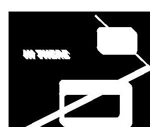
    Eg: >> B = ones(3);
        >> BWE = imerode(BW,strel(B));
        >> imshow(BWE)

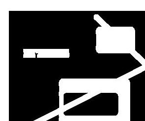
      Eroded image BWE      Twice-eroded: add the code line
                            >> imshow(imerode(BWE,strel(B))
  

      In this example, a foreground pixel "survives" an
     
    erosion only if there is a 3x3 square of white
     
    pixels below it and to its right. So the diagonal
     
    lines thin from an original thickness of 4 pixels
     
    to 1 pixel with the first erosion, then disappear
     
    with the second erosion.

    Erosion and dilation can be used to perform many

    useful image processing tasks. They can be used

    together and in combination with standard binary

    set operations such as set difference:
 

                  X / Y = X and Y^c
 

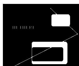
    Eg: Erosion followed by set difference yields the

        interior boundary.

        >> IB = BW & ~BWE;
        >> imshow(IB)
 
 

        Similarly, dilation followed by set difference

        yields the exterior boundary.

        >> EB = BWD & ~BW
 

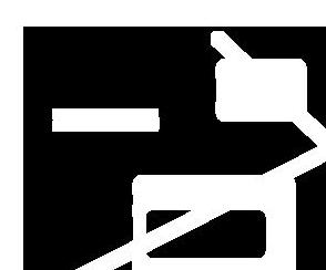
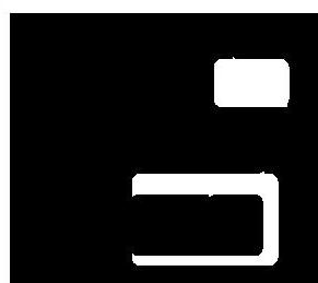
    Erosion followed by dilation is called opening.

    Opening breaks weak connections between blobs. It also

    eliminates small features while leaving larger ones

    unchanged.

      Eg:

        >> SE=strel(ones(3));
        >> BWO=imdilate(imerode(BW,SE),SE);
        >> imshow(BWO)
 

       Original image BW         BW after opening operation
 
 

    Eg: Dilation followed by erosion is called closing.

        Closing connects up distinct blobs that are near

        one another, also smooths out rough boundaries.

        >> BWC=imerode(imdilate(BW,SE),SE);
        >>imshow(BWO)

    BW closed by SE=ones(3)     BW closed by SE=ones(7)
 

    Note how the isolated fragments are glued together by

    the closing operator. But bigger objects are not

    changed, note the lack of distortion of the big blobs.
 
 

Graphical notation for representing images and

structuring elements

Mark each image point with a dark square, and mark

the origin (0,0) with an X ("ex").
 

Eg: B1={(1,1),(-1,1),(1,-1),(-1,-1)},

    B2={(0,0),(1,0),(2,0)}

Dilation: for each (i,j) in input image X,

    1. Align ex in B with (i,j)

    2. Mark each y under a dark square in B as a dark

       square in Y, i.e a pixel in the dilation Y=X(+)B.

Erosion: for each (i,j) in ZxZ,

    1. Align ex in B with (i,j)

    2. If every dark square in B is aligned with a

       dark square in X, them mark (i,j) as a dark

       square in Y, i.e. a pixel in the erosion Y=X(-)B.
 

Eg: Using B1 and B2 above,

Other definitions and formal properties:
 

A morphological transformation psi is a mapping

psi:X->Y where X and Y are point sets (subsets

of ZxZ). Quantitative transformations psi have

four explicit properties described in the text.

All the morphological transformations we shall

study are quantitative.
 

The dual of a morphological transformations psi

is defined as the psi* such that for all X,

psi*(X) = [psi(X^c)] ^c

    Eg: erosion and dilation are dual operations,
    as  are opening and closing.

 

CSE573 Fa2010 11-15

---

 

Properties of dilation:
 

1. Commutivity: X(+)B=B(+)X

2. Associativity: X(+)[B(+)D]=[X(+)B](+)D

3. Translation invariance: X_h (+)B=[X(+)B]_h

Note subscript means translation by h.
 

4. Increasing: X contained in Y implies

   X(+)B contained in Y(+)B

5. Extensive if (0,0) in B: X(+)B contains X
 
 

CSE573 Fa2010 11-16

---

 

_{Properites of erosion:}
 

1. Not commutative: X(-)B~=B(-)X

2. Not associative: [X(-)B](-)D~=X(-)[B(-)D]

   In fact, [X(-)B](-)D=X(-)[B(+)D]

3. Translation invariance: X_h(-)B=[X(-)B]_h

4. Increasing: X contained in Y implies

   X(-)B contained in Y(-)B

5. Anti-extensive if (0,0) in B: X contains X(-)B
 
 

CSE573 Fa2010 11-17

---

 

_{Gray-scale morphology}
 

_{So far we have defined all psi-operations}

_{(eg. dilation, erosion, opening and closing)}

_{only on binary images, those that can be}

_{represented by unattributed point sets in ZxZ.}
 

^{In the case of gray-scale images, we define}

^{an image to be a pointset from ZxZxG, where}

^{G is the set of possible gray-scale values.}

^{G can be {0..255} for 8-bit images, [0,1] for}

^{real images, or even {0,1} for binary images.}

^{Thus gray-scale images are sets of triples, not}

^{doubles as for binary images.}
 
 

CSE573 Fa2010 11-18

---

 

^{Eg: X={(1,-1,114),(2,-1,128),(3,-1,101),(2,-2,74)}}

    ^{B={(0,0,62),(1,0,55)}}

Gray-scale Dilation : Let x(i,j) be the gray level

at (i,j) in the input image X. Then Y is the

gray-scale dilation of X iff
 

    y(i,j)=max [x(i-n,j-m)+b(n,m)]
 

where the max is taken over all (n,m) in the

support of B and (i-n,j-m) in the support of X.
 

    Notes: 1. (n,m) in the support of B means
              that B(n,m) is not equal to 0.

           2. If G in X is bounded then y inherits
              the same bounds on G.
 
 

CSE573 Fa2010 11-18

---

 

 

CSE573 Fa2010 11-19

---

Gray-scale Dilation: geometric interpretation

In 11-14 above we introduced a way of computing

dilation and erosion geometrically. Here is that

approach extended to gray-scale dilation:
 

    1. Flip B left-right and top-bottom around its

    origin, the pixel marked with an ex. Call this

    new structuring element B' (B'(i,j)=B(-i,-j)).
 

    2. Align B' with the original image so that

    the origin ex in B' is over some arbitrary

    pixel (i,j) in the original image. Then the

    corresponding pixel (i,j) in Y will be non-

    zero if and only if some non-zero pixel in

    B' is aligned with a non-zero pixel in the

    original image. Its value will be the maximum

    sum of pairs of aligned pixels.
 

CSE573 Fa2010 11-19a

---

Eg: See the example above. B' corresponds to B

    above except the pixel of value 55 is to the

    left of the pixel marked with "X" and 62.

    Then if, for instance, we align B' so that

    its origin is over the pixel of value 101,

    which is at (i,j)=(3,-1), we will have
 

        Y(3,-1)=max(55+128,62+101)=183
 

    And if we align it over (i,j)=(3,-3) we will

    have Y(3,-3)=0 since neither non-zero value

    in B' is aligned with a non-zero value in

    the original image. Proceeding this way we

    can align with all pixels (i,j) and compute

    the gray-scale dilated image Y.
 

CSE573 Fa2010 11-19b

---

 

Gray-scale Erosion: for each (i,j) in ZxZ,
 

    y(i,j)=min [x(i+n,j+m)-b(n,m)]
 

where the min is taken over all (n,m) in the

support of B. 
 

Notes: 1. As before, y inherits G's bounds.

       2.(n,m) is in the support of B iff

         B(n,m) ~= 0.

Geometrically, align B with the original image so

that the origin ex in B is over some arbitrary

pixel (i,j) in the original image. Then the

corresponding pixel (i,j) in Y will be the minimum

difference of pairs of aligned pixels.

 

Eg: Using X and B above, let Y = erosion of X by B:

 

There is an interpretation of gray-scale morphology

operations in terms of the umbra and top

surface structures. The resulting operations

are identical to those described algebraically.

above.

Define the umbra U of a gray-scale image X=(x,y),

x in R² and y in R¹ , as the point set in R³ which is

bounded above by X, ie.
 

    U(X)={(x,y') for (x,y) in X and y'<=y}.
 

Also define the Top Surface T of a gray-scale image

X as the point set in R³ which bounds X from above,
 

    T(X)={(x,y) in X such that for all (x,y')

    in X, y>=y'}
 

Then the 3D-geometric interpretation of the gray-scale

dilation Y of X by B is that it is the top surface of U(Y),

where U(Y) is the binary dilation of U(X) by U(B).

Note this is binary dilation in R³.
 

The construction of the gray-scale dilation Y of X using

the structuring elemement B and following this interpretation

goes like this:
 

    1. Construct the umbras U(X), U(B).

    2. Align the ex in U(B) with a element of U(X).

    3. Mark all cells occupied by U(B) cells as

       U(Y) cells.

    4. Repeat 2 and 3 for all elements of U(X),

       yielding U(Y).

    5. The top surface of U(Y) is the desired dilation.
 
 

Example: using the same X and B as before,

First align (0,0,0) of U(B) with (1,-1,0) of U(X). Mark

all U(X) cells which are covered by U(B) cells, namely

the 63 cells (1,-1,0)..(1,-1,62) and the 56 cells (2,-1,0)..

(2,-1,55), plus all cells below these cells, as belonging

to U(Y).
 

Next align (0,0,0) of U(B) with (1,-1,1) of U(X). Repeat.

Get two additional cells in U(Y): (1,-1,63) and (2,-1,56).
 

Keep going like this. End up with the U(Y) shown in top

view as

To get the top surface, just strip away all cells except

those with the highest y-values for any x in U(Y). This is

the gray-scale dilation of X by B.

A corresponding procedure works for constructing the

gray-scale erosion of X by B:
 

    1. Construct the umbras U(X), U(B).

    2. Align the ex in U(B) with a cell (i,j,k).

    3. If every cell in U(B) is aligned with a cell in U(X),

       mark cell (i,j,k) as an element of U(Y).

    4. Repeat steps 2 and 3 for each (i,j,k) in R³

       yielding U(Y).

    5. The top surface of U(Y) is the desired erosion. 

The 2D-geometric interpretation or the 3-D geometric

interpretation lead to algorithms of similar computational

complexity. Of course, the resulting erosions and dilations

are identical whichever is used.

Other gray-scale morphological operations:
 

Opening and closing are defined identically to binary case,

but the "overloaded" erosion/dilation operators are in this

context interpreted as gray-scale erosion/dilation.
 

       Opening: [X(-)B](+)B  

       Closing: [X(+)B](-)B

       where (-) and (+) are grey-scale operations

 
We know that binary opening kills small foreground blobs

and breaks weak links between blobs. Gray-scale opening is

a "soft" version: it darkens small blobs and narrows weak

links. Similarly, gray-scale closing brightens small blobs

and creates links between near-by blobs, and brightens

isolated blobs.

Top-hat transformation
 

Recall that we defined the set difference X\Z as the

elements of X that were not in Z, X\Z = (X and Z^c).

The top-hat transformation is the set difference

between an original image X and its opening, ie
 

        Top-hat: X\{[X(-)B](+)B}
 

Since opening an image eliminates small regions of

high local contrast, the Top-hat transformation finds

such small regions and eliminates the background. So

slowly varying background behind bright (or dark)

objects is eliminated.
 

Skeletons and other morphological descriptors
 

Binary objects with complex shapes can often be

represented by simple skeletons. Skeletons capture the

shape of an object, but in a more compact form than

the full object itself.
 

Define a ball B(p,r) as a set of points {x} in a binary

image such that d(p,x)<=r. The distance metric used

determines the shape of the ball.
 

Eg: p=(10,10), r=3.

 

A maximum ball of a connected binary set (object) X

is a ball B contained in no other ball in X.
 

The maximum-ball skeleton S(X) of X is the set of all

centers p of maximum balls B(p,r) in X.
 

Eg: 8-connected maximum-ball skeletons of the black

    objects shown as empty squares. Note: in these

    examples, the empty squares were all originally

    black, ie. are parts of the object.

A problem with the maximum ball skeleton S(X) is that

if the object X is not convex, its maximum ball skeleton

S(X) may consist of disconnected segments. Homotopic

skeletons are skeletons which preserve the desirable

property of connectedness. Homotopic skeletons can be

produced using the thinning operator X(/)B.
 

Define the Hit-Or-Miss Transformation (x) of X relative

to a pair of structuring elements (B₁,B₂) as
 

        X(x)B = {x in X(-)B₁ and X^c(-)B₂}

where B=(B₁,B₂).
 

In other words, a point x survives (x) if, when you

align the origin of B₁ at x, all points of B₁ match

X points, and when you replace B₁ by B₂, no points of

B₂ match X points.
 

Now lets define thinning and thickening in terms of (x):
 

    Thinning (/):   X(/)B = X\(X(x)B)

    Thickening (*): X(*)B = XU(X(x)B)

  In other words, we find the pointset in X that perfectly

matches B, X(x)B, and remove it from X to get the thinned

version X(/)B, or add it to get the thickened version

X(*)B. If B2 is not empty, then the perfectly matched

portion X(x)B will be on the boundary of X.
 

Using a sequence of thinning operators with different

orientations, we can reduce the thickness of an object

uniformly. Continuing to do this until no further

pixels are lost, we have the homotopic skeleton.

See text p 579-8 for details.
 

Quench function
 

Give the maximum-ball skeleton of an object, if we

knew the size of the maximum ball for each skeleton

point we could reproduce the original object exactly.

Let S(X) be the maximum-ball skeleton of a binary

image X and p be a point in S(X). Define the quench

function q_x(p) as the size of the maximum ball in

X at p. Then X can be reconstructed from (S,q) by
 

        X = U [p + q_x(p)B]

where the union is over all p in S(X).
 

Eg:

One important use of the quench function is to define

the ultimate erosion of an object. If one tries to

iteratively erode a figure to get a skeleton, problem

is that parts of the skeleton disappear too. This is

particularly a problem for non-convex objects.
 

The ultimate erosion of X is defined as the union of

all the regional maxima of the quench function.

The regional maxima {M_i} are connected regions of

uniform gray value such that all neighbors of M_i

have strictly lower gray value (note that gray value

refers to the value of the quench function).
 

So the ultimate erosion consists of high flat

ridges and plateaus in the maximum-ball skeletons.
 

  Eg: Ultimate erosion shown in black

Granulometry
 

Given an image containing a set of blobs, it is often

of interest to tabulate blob size distributions.
 

Eg: In an image of oil droplets from an automobile

    engine, we want to determine the distribution of

    sizes of metal shavings. We may measure size by

    area, by chord length,or some other way.
 

Eg: In an image of particulate matter captured from a

    "clean room" for VLSI chip manufacture, we may

    need to certify how many particules >50 micrometers,

    between 20 and 50 micrometers, <20 micrometers.
 

The blob count as a function of blob size is called the

granulometric curve.
 

Eg:

The granulometric curve can be computed by segmenting the

image, then computing the desired size metric for each

segment separately. But this is very computationally

expensive, particularly for images with many blobs.
 

Morphologic approach to the granulometric curve
 

Consider a set of increasing, anti-extensive openings

{psi_n, n=1,2...}. This set of openings is called a

granulometry .
 

For each opening psi_n, assume we will use the same

structuring element for both the erosion and dilation

parts of the operation. Call the common structuring

element B_n. Typically B_n is just a scaled version 

of B_n-1.

As we iteratively open an image with {psi_n, n=1,2...},

the original blobs get smaller and eventually disappear.  

Label each pixel p in each blob with the n at which

that pixel disappears from its blob. The resulting

gray scale image is called the granulometry function

G_psi(X).

Note: In visualizing the opening operation, there is a

useful geometric interpretation. The opening X(-)B is the

footprint of B as it is translated everywhere inside each

blob in X in which it fits.
 

Eg: Let B_n be an nxn square structuring element.

The next opening, X(-)B1(-)B2(-)B3(-)B4, is empty.

So lets create the granulometry function G_psi(X):

The histogram of this image is the granulometry curve

of the original image X with respect to the granulometry

{psi_n, n=1,2...}. Often this histogram is relabelled to

indicate structuring element B_n size on the horizontal

axis and pixel count divided by the size of Bn on the

vertical.
 

Eg (continued):

Note on the right graph that the area of Bn is greater

than the area of the particles that disappeared using

Bn. So this means that there are ~5/2 particles of

size 1-3 pixels, ~10/9 particles of size 4-8 pixels

and ~9/16 particles of size 9-15 pixels.
 

Morphological segmentation
 

Segmentation is particularly difficult when you are

working with many distinct but similar objects, such

as a bowl of gumballs, a honeycomb, or a soap-bubble

foam. For such gray scale images, segmentation by

watersheds works well. Binary images can be converted

to gray scale for this purpose using the distance

function dist_X(p).
 

Let X be a binary image and B a structuring element.

For each point p in X, define the distance function

dist_X :X->Z by
 

    dist_X (p) = min {n such that p not in X(-)nB}
 

In other words, for each pixel mark that pixel by the

number of times opening by B must be done before p

disappears from X.
 

Note the similarity between the distance function and the

quench function described earlier. The quench function is

the distance function defined on the maximum-ball skeleton

when the unit ball structuring element is chosen.
 

The idea here is to use the negative distance function

-dist_X(p) as a gray scale image and do the usual watershed

segmentation on that image. That is, fill catchment basins

from the bottom of the lowest one. Where two basins touch

at equal values of gray scale, mark a "dam" or segment

boundary between them (see Section 5.3.4).