CSE473/573 Fall 2010 Lecture Charts
Chapter 3: Data structures for image
analysis
Matrices
The most common data
structures for images are 2D
arrays, ie. matrices,
whose pixel values represent
brightness
information. For an n row by m column
image, M:
{1,..,n}x{1,...,m} -> V.
V=B={0,1}: binary image
V={0,...,2b-1}: b bit intensity
image
In case of a color image, three
matrices may be
used corresponding to
RGB, CMY, YIQ, HSI, or
some other color
model
(Matlab refers to any
color image as an RGB image).
Indexed Image
Alternatively, an image can be described by
a combination of a
look-up table (LUT) and a
matrix of values
pointing to it. This is called
an indexed image.
For a color image,
each LUT entry is set
of three
numbers, the color
values
associated with the entry.
There may be any
number of distinguishable colors
in the LUT.
The LUT is also
called a color
map
CM, and the
combination of the
LUT and the matrix of index values
is the indexed image.
V={0,...,2b-1}: b bit indexed image
CM:
V -> C, a set of distinguishable colors.
Eg: In an 8-bit color
image, pixel value V=23 may
be indexed to the
color C=(255,0,0) or bright red.
An 8-bit indexed
image
has a pallette of 256
colors, a 24-bit
image
can map 224 = 16M colors.
Matrices have limitations as data
structures. They
tend to store images very redundantly,
images which
can be easily compressed without loss of
accuracy.
They also do not capture shapes or regions
very
efficiently. Here are some other data
structures
useful for representing all or parts of
images.
Chain codes
These are useful in
defining linearly connected
sets (each pixel has
no more than two neighbors).
Eg:
Starting top
row left, a 4-neighbor chain
code of the
border of this
blob is EESESEWWWSWNWNEN. An
8-neighbor
code would be
E/E/SE/SE/W/W/SW/W/NW/N/NE.
Run length codes
Image representations
useful for compression of
binary images. The
beginning and end of runs are
coded.
Eg: Consider the
small binary image
RLCode =
((row1code)(row2code)...)
Rowcode =
(Rownum, BRS1, BRE1, BRS2, BRE2,..)
where BRSn means Black (binary 0) Run n Starts
BREn
means
Black
Run
n
Ends
RLC for this
image is
((1)(2,5,6)(3,4,4,7,7)(4,4,4,7,7)(5,5,6)(6))
Graphs
Relationships like
"segment 5 is adjacent to segment 12"
or "the image of the
man is near the image of the tree"
are often represented
by graphs.
There are many kinds
of graphs (eg. directed, undirected,
attributed, trees of
various kinds) to represent different
relationships.
Eg: adjacency graph
(unattributed, undirected)
We could make this
graph attributed by putting segment
characteristics
inside
the nodes, for instance "flat,"
"curved," numerical
vector value of the outward pointing
normal, etc.
We could make it directed by having
edges correspond
to some
non-commutative binary relation such as
"is closer to
viewpoint than" or "is bigger than."
Pyramids
Often it is necessary
to analyze scenes at multiple
levels of resolution
simultaneously. Pyramids are
data structures well
suited for multiresolution
image processing.
Eg: Picking up a pen
you just dropped. You need to
see the space between
you and the pen in low-res to
avoid collisions, the
floor in medium-res to guide
your arm to the
vicinity of the pen, and the pen in
high-res to direct
your fingers to a secure grasp.
Eg of a
multiresolution image (foveal format) and its
uniform resolution
component subimages.
A Matrix-pyramid
(M-pyramid) is a set {ML,...,M0} of L+1
images derived from a
single 2Lx2L gray level image ML.
ML-1 is
derived by averaging four adjacent child nodes
in ML to
compute one parent node. ML-1 is of dimension
2L-1x2L-1.
The
four-child
averaging
continues
to
M0, of
dimension 1x1, the
"grand average" of all pixels in ML.
Eg: M-pyramid for a
8x8 3-bit image
using roundoff
truncation:
M3: 2 4 7 0 0 2
6 3 M2: 2 2 2 5 M1: 2 4 M0: 3
3
0
0
1
1
3
6
4
2
1 2
5 3 4
2
2
0
1
1
4
6
3
4
1 3 5
3
2
1
1
1
2
6
3
5
1 2 6
4
3
1
1
2
3
6
3
4
4
2
1
2
4
7
5
5
4
2
1
1
4
7
5
5
5
1
0
0
2
7
5
This is called
an "averaging M-pyramid." Other functions
of the four children
can
be used to define the parent
node's value, for
instance parent =
max(children) or
parent=median(children).
Also,
9
instead
of
4
children
can be used,
resulting in a more compact M-pyramid such
that each higher
layer is 1/9 as big as the next lower
rather than 1/4 as
with the 4-child M-pyramid. We
can also have an
"overlapping M-pyramid," in which each
child can
have more than one parent.
A related data structure is the Tree-pyramid
(T-pyramid)
which relates all nodes to a common tree.
Eg: The T-pyramid for the image M2:
V: (L,R,C) -> G where L is the M-pyramid
level (0 is top
level), R and C are the M-pyramid row and
column indices,
and G is the graylevel value of that node.
Notice in a standard, non-overlapping
T-pyramid each
parent has
exactly 4 children regardless of the image
contents.
Thus a T-pyramid often contains much redundant
information.
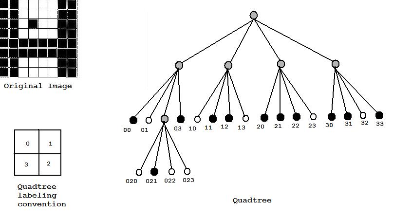
A Quadtree
is a compressed form of a T-pyramid. Starting
from the full-resolution level L, if all 4
children of a
given parent on level L-1 are identical,
then these four
nodes on level L are deleted from the tree.
If for
instance the top-left quadrant of a
given image
is constant, it will be represented by just
one node
in the quadtree, not a subtree of nodes
with root at
that node.
Eg: Consider the
quadtree representation of an 8x8 binary
noisy image of the letter H shown below. Each leaf
of the
quadtree contains
three kinds of information: the
location
of the pixel set
it corresponds to, the number of
pixels,
and the color
(black or white).
Matlab and the Image
Processing Toolbox
We will be using Matlab frequently this
semester as
a tool for exploration and visualization.
To
start
Matlab from the unix prompt (>), type
> matlab
When you see a new window pop up with a
subwindow
showing a double-caret prompt (>>) Matlab is
ready to accept commands. Matlab is
available on
the CIT, CSE and ENG Linux/Solaris domains. Matlab
is not available on any of the UB Windows networks.
The basic Matlab commands will be discussed
in
recitation. Tutorials and user's guides are
available
on the
web, see our newsgroup sunyab.cse.573 for some
links.
The Matlab commands that are specific to
image work
are located in the Matlab Image Processing
Toolbox,
/util/matlab/toolbox/images/. You can see a
list
of all IP Toolbox commands, from the UNIX
prompt,
> more
/util/matlab/toolbox/images/images/Contents.m
To access online help on any matlab command
say the
command "command_name," type
>> more on
>> help command_name
Check sunyab.cse.573 for a list of urls
containing
tutorial and reference information for
Matlab and the
Image Processing Toolbox.
Image types supported
by the IP Toolbox
There are 4 image types Matlab supports.
All
of them
are matrices or sets of matrices. The data
in these
matrices are either of type double
(floating
point
double precision) or uint8 (unsigned byte
{0...255}).
1. Intensity image: matrices of type double
normalized
to [0,1], or of type uint8. These are
graylevel images.
In a double normalized image 1.00 is pure
white 0.00 pure
black. In a uint8 image file, 255 is pure
white 0
pure black.
Eg: 4x4 double intensity image INT =
0.66 0.31 0.01 0.14
0.25 0.91 0.04 0.19
0.22 0.92 0.11 0.67
0.29 0.77 0.17 0.40
Eg: 4x4 uint8 intensity image INT =
122 105 116 070
131 100 090 044
158 101 040 020
201 115 021 003
2. Binary image: matrices of type double
normalized
[0,1], type uint8 logical
({0,1}) or uint8 non-
logical ({0,255}).
Eg: 4x4 binary double normalized
[0,1]:
1.00 1.00 1.00 0.00
1.00 0.00 1.00 0.00
1.00 1.00 0.00 0.00
0.00 1.00 1.00 0.00
Eg: 4x4 binary uint8 logical
1 1
1 0
1 0
1 0
1 1
0 0
0 1
1 0
Eg: 4x4 binary non-logical
255 255 255 0
255 0 255 0
255 255 255 0
0 255 255 0
3. RGB image: NRxNCx3 arrays of type double
normalized
[0,1] or uint8. RGB(:,:,1) is
the 'red' intensity
image, RGB(:,:,2) the 'green'
and RGB(:,:,3) the
'blue'.*
These are "truecolor" 24 bit images.
4. Indexed image: An indexed image consists
of a NRxNC
data matrix and a NPx3 color
map. The data matrix is
of type double normalized
[0,1]
or uint8, the color
map is double normalized
[0,1].
The data matrix
values are row pointers to the
color map RGB values,
{1...256}. Indexed images are
color images with a
limited palette of NP colors
(out of 224).
Eg: In an indexed image, suppose
data pixel
(10,33) has value
114.
If
row 114 of the
color map
has value
(0.00,1.00,0.00) then
pixel
(10,33) will be painted
bright green.
* Note:
A
colon
":"
as
an
index
argument
in
matlab
means
"all values of this index." So for instance given a 4x4
matrix M, M(:,2) would be all the data stored in
column
2 of M. This would be a 4x1 column vector. And in a
256x256x3
truecolor
image
with
filename
IM,
IM(:,:,1)
would
be
the
256x256
matrix
consisting
of
the
red
values
in
IM.
Image input
You can create an image from the keyboard by
creating a matrix or set of matrices as
above.
Eg:
>> BW=[1 0 1;1 1 0] creates a 2x3 BW
type
double image.
To import an external (non-Matlab) image
format
such as jpg or tiff or bmp, etc., to one
of the internal Matlab-supported image types
above, use the command imread. An example
use is:
>> FOO=imread('foo.jpg','jpg')
If foo.jpg is a NRxNC jpeg image, then FOO
will
be a NRxNCx3 Matlab uint8 RGB image.
For importing an indexed image type such as
a gif
file *.gif or an X-window dump files *.xwd,
the
syntax is
>> [FOO,CM]=imread('foo.xwd','xwd')
Then FOO is the data matrix and CM the
color
map.
Image type conversions
Once a Matlab image has been imported or
created,
it can be converted to another Matlab image
type.
im2bw, im2uint8, and im2double are commands
which
convert any Matlab image to bw, uint8 or
double.
Indexed images are converted from other
formats
using the
commands gray2ind, grayslice, rgb2ind,
dither. Use
the help facility to see the specifics.
Eg:
>> INT=[0.8 0.6 0.4; 0.1
0.0 0.1; 0.5 0.5 1.0]
creates a 3x3 double normalized
[0,1]
array,
which is a Matlab intensity image of
type double.
>> BW=im2bw(INT,0.5)
produces a 3x3 binary uint8 array BW
1
1 0
0 0
0
1 1
1
The 0.5 argument is the black-white
threshold.
BW can be then converted back to type
double by
>> BW=im2double(BW)
These conversion routines rescale and shift
as needed
to comply with the converted image
requirements. Note: you
can convert uint8 <-> double using
typecasts. But you may
not end up with a normalized image.
Eg:
Image display:
use the imshow command.
Eg: >> BW=[zeros(50,50)
ones(50,50)];
>>
GR=[.75*ones(50,50)
.25*ones(50,50)];
>> INT=[BW;GR];
>> imshow(INT)

Imshow(IND,CM) will display the indexed
image IND
using the color map CM.
Image output:
to export an image in an external image
format such as jpg or tiff etc., use
imwrite.
Eg: Continuing the previous example,
>>
imwrite(INT,'squares.jpg','jpg')
stores the Matlab
intensity image INT as a jpeg
file squares.jpg.
Notes
1. Cannot do arithmetic on uint8 data.
Convert to
type double, then do
arithmetic, then convert
back. Can use typecasts
double()
and uint8().
Eg: We have a uint8 image INT
which we want to
scale
to {0...63}.
>>
INT=double(INT)/4;
>>
INT=uint8(floor(INT));
2. Any toolbox function that returns a BW
image by
default returns a BW image
uint8 {0,1}
with its
logical flag on. This permits
the image to display
properly. If a uint8 {0,1}
image is
created any other
way its logical flag by
default is off
and
imshow
will look solid black.
logical() turns
the flag on,
+ off.
Eg:
>> BW=uint8([ 1 0 1;
0 1 0; 1 0 1]);
>>
BW=imresize(BW,100);
A 3x3
pixel image can't be
seen
on the display,
there
is not enough contrast between grey level
0 and
grey level 1 (out of 255). So we turn the
logical flag on before displaying it.
>>
imshow(logical(BW))