Goals of Pre-processing:
 

1. Noise and clutter reduction.

   Noise: random errors in pixel values

   Clutter: unuseful image components
 

2. Imaging model compensations.

   Geometric distortion, color imbalance, graylevel

   distortion, fixed pattern distortion.
 

3. Feature enhancement.

   Edge enhancement and smoothing, histogram

   equalization, falsecolor coding.

Pre-processing tends to be local and hardwired.
 

 Local: mapping at (i,j) depends only on

 values near  (i,j).
 

 Hardwired: not content, context or task

 dependent. Invariant.

    CSE573 Fa2010 Peter Scott 04-01

---

Pixel brightness transformations
 

Due to different sensitivities of each pixel in the

camera to the light that hits it,
 

                f(i,j) = e(i,j) g(i,j)
 

where g is the ideal scene brightness, f the recorded

image brightness, and e a matrix of error

coefficients.
 

e(i,j) is called pattern noise. Easiest way to

determine pattern noise is to view a uniform scene

such as a white sheet of paper. Then g(i,j)=c and
 

            e(i,j) = f(i,j)/c
 

Pattern noise can be compensated by differential

scaling of each pixel
 

            f_p(i,j) = f(i,j)/e(i,j)
 

This can be done with a LUT and dedicated multiplier



            LUT(i,j) = e^-1(i,j).
 

    CSE573 Fa2010 Peter Scott 04-02

---


Grayscale transformations
 

Let P be a set of scalar pixel graylevel values

(P=[0,1] or R¹ or {0...255} etc.). Then T:P->P

is a grayscale transformation. T maps each graylevel

to a new graylevel separately and  independently.


Egs:

 

CSE573 Fa2010 Peter Scott 04-03

---

Another grayscale transformation is histogram

equalization. The goal of histogram equalization

is to have an equal number of pixels at each

graylevel in P, the set of permissible graylevel

values. A histogram equalized image uses the

P as efficiently as possible, maximizing the

entropy of the image.
 
 

First count the pixels residing at each of the G

possible graylevels in the input image. This is the

histogram. Then compute how to reassign pixel values


so that the histogram is as spread out as possible.

CSE573 Fa2010 Peter Scott 04-04

---

The algorithm is given in the text on p 61:


        T(p) = round(((G-1)/NM)H_c(p)), p=0,...G-1


where the image is NxM with G grey levels 0..G-1, H_c(p)


is the cumulative histogram and T(p)=q means reassign


the pixels of grey level p in the original image to


grey level q in the equalized image.


A cumulative histogram for each k sums all the values


in the (normal) histogram for greylevels less than or


equal to k.



Eg:


 

CSE573 Fa2010 Peter Scott 04-05

---

T(0)=round((7/100)H_c(0))=round(0)=0,  old 0 pix -> 0 pix


T(1)=round((7/100)H_c(1))=round(.7)=1, old 1 pix -> 1 pix

T(2)=round((7/100)10)=round(.7)=1,    old 2 pix -> 1 pix 

T(3)=round((7/100)10)=round(.7)=1,    old 3 pix -> 1 pix


T(4)=round((7/100)27)=round(1.89)=2,  old 4 pix -> 2 pix


T(5)=round((7/100)49)=round(3.43)=3,  old 5 pix -> 3 pix


T(6)=round((7/100)74)=round(5.18)=5,  old 6 pix -> 5 pix


T(7)=round((7/100)100)=round(7)=7,    old 7 pix -> 7 pix


CSE573 Fa2010 Peter Scott 04-06

---


 

Eg (cont'd):



Notice that the histogram equalization is not

perfect (each bin having equal occupancy would

be perfect). But there is better use of contrast


since the pixels are more spread out in greylevels.
 

CSE573 Fa2010 Peter Scott 04-07

---


 

Geometric transformations x'=T_x(x,y), y'=T_y(x,y)
 

Changes in scale, shifts and rotations of images

can be done using geometric transformations Tx,

Ty called affine transformations:
 

         [xp;yp]=T*[x;y]+[a0;b0]
 

Note: where plain rather than bold face is used

     as above this signifies Matlab notational

     conventions are being used.
 

Eg: Rotate image by 30 degrees ccw and shift

    resulting image 2 pixels to the right.
 

   T=[cos(pi/6) -sin(pi/6); sin(pi/6) cos(pi/6)]

   a0=0

   b0=2

CSE573 Fa2010 Peter Scott 04-08

---


 

To rotate the image cw, use negative angle. To rotate

around point (x0,y0) rather than (0,0),

    1. Shift image by (x0,y0): T=I, a0=-x0, b0=-y0

    2. Rotate: T=[cos -sin; sin cos], a0=b0=0

    3. Shift back: T=I, a0=x0, b0=y0
 

CSE573 Fa2010 Peter Scott 04-09

---

Interpolation
 

A difficulty with geometric transformations

is that in general the transformed image

locations (x',y') are not on equi-spaced

grid points (raster) that the original

image samples (x,y)=(i*deltax,j*deltay)

were. We compute the new values on this

raster by interpolation.
 

Let (x',y') be a point on the raster whose

transformed value we wish to compute. Let 


        [x;y] = T^-1*([x';y']-[a0;b0])


 


be the coordinates of this point back in the

original image. Now we will interpolate the

neighboring raster values in the original

image to get the value at (x',y').
 
 

CSE573 Fa2010 Peter Scott 04-10

---

Eg: 30 degree cw rotation around x=y=0, with

    image raster (x,y)=(i,j), i=1..NR, j=1..NC
 

        T=[.866 .500; -.500 .866]
 

    Lets compute for instance the value of the

    rotated image at the raster point (4,2).
 

        T^-1*[4;2]=[2.46;3.73]
 

    So we want to interpolate to find the value

    of the original image at (x,y)=(2.46,3.73).

    Assume that in the original image, the

    surrounding gray level values are



            g_s(2,3)=115, g_s(2,4)=144

            g_s(3,3)= 82, g_s(3,4)= 65







 
 
 
 
 

CSE573 Fa2010 Peter Scott 04-11

---


 

Now there are several interpolation rules we

can use. Nearest neighbor interpolation assigns

to the unknown point the value of the closest

raster point. In the example this would be
 

   f₁(x,y)=g_s(round(x),round(y))=g_s(2,4)=144.

   g_s1(x',y')=f₁(x,y)
 

Here g_s(x,y) is the original sampled image

defined for raster values of (x,y), f₁(x,y)

are the values of the original image off the

raster, and g_s1(x',y') is the transformed

image defined for raster values of (x',y'),

and round(x) rounds to nearest integer.
 
 

CSE573 Fa2010 Peter Scott 04-12

---


 

Linear interpolation assigns to the unknown point

a weighted average of the values of the four

nearest neighbors as follows: let a=x-floor(x),

b=y-floor(y). Then
 

 f₂(x,y)=(1-a)(1-b)g_s(l,k)+(1-a)(b)g_s(l,k+1)+

        +(a)(1-b)g_s(l+1,k)+(a)(b)g_s(l+1,k+1)
 

In this formula, l=floor(x) and k=floor(y). As

before, g_s1(x',y')=f₁(x,y) sets the transformed

value on the raster point (x',y'). floor(x)

rounds down.
 

CSE573 Fa2010 Peter Scott 04-13

---


 

Eg (continued):

    Interpolating the point (x,y)=(2.46,3.73)

    using linear interpolation, we have a=.46,

    b=.73, l=2, k=3 and
 

    f2(x,y)=.54*.27*115+.54*.73*144+

           +.46*.27* 82+.46*.73* 65

           = 105.54

    If this is a uint8 image, we would quantize

    to graylevel 105.

Note that the two different interpolation rules

lead to quite different results: 144 vs. 105.

Linear leads to smoother transitions, nearest

neighbor interpolation is faster.
 

    CSE573 Fa2010 Peter Scott 04-14

---


 

There are other more accurate interpolation methods,

for instance bicubic interpolation (text eqn. 4.23).

This method uses a non-linear average of 16 pts. For

most imaging tasks, linear interpolation works ok.

For high-precision work such as special effects for

the movie industry, bicubic interpolation is done.
 
 
 

CSE573 Fa2010 Peter Scott 04-14a

---


 

Local preprocessing: filters
 

One useful class of preprocessing operations is to

multiply the image pixels by mask values and sum

over the mask.
 

Eg:  Mask h: 1 2 1 (*1/20)   Image g: 1 1 1 1
             2 4 2                    1 6 1 1
             1 2 1                    0 1 0 1
                                      1 1 7 0

     Mask origin: h(2,2)



    First step: Zero-pad the image so mask fits

    over every pixel. That is, add row/columns

    of zeros borders to the given image so that


    when the mask origin is aligned with any pixel


    in the image, the mask pixels do not extend


    beyond the zero-padded image.



    In the case of a 3x3 mask with mask origin in the


    center of the mask, the border needs only

    to be zero-padded by a single row/column all around.
 

     Padded image:   0 0 0 0 0 0
                     0 1 1 1 1 0
                     0 1 6 1 1 0
                     0 0 1 0 1 0
                     0 1 1 7 0 0
                     0 0 0 0 0 0
 

CSE573 Fa2010 Peter Scott 04-15

---


 

    Second step: Repeat for each pixel (i,j) in the


    original image (not the zero-border pixels):


    center the mask over (i,j) in the original image


    and compute the  sum of products of



         (mask values * aligned pixel values)



    Enter this value into pixel (i,j) in the


    new "filtered" image.
 

          Final image f: 14 22 17  9 (*1/20)
                         20 34 24 11
                         13 28 28 14
                          7 22 32 16
 

This multiply-sum-shift operation is called

convolution of the image by the mask (convolution

kernel). The result is called a filtered version

of the original image. For each pixel (m,n) in the

image g(m,n) to be filtered using mask h(k,l), the

filtered image f(i,j) is given by

CSE573 Fa2010 Peter Scott 04-16

---


 

The amount of zero-padding that has to be done depends

on both the size of the mask and where on the mask the


mask origin is located.



Eg: Previous example, 3x3 mask with origin in center,


    need to zero pad with a single row or column on all


    four sides of the image:



                     0 0 0 0 0 0
                     0 1 1 1 1 0
                     0 1 6 1 1 0
                     0 0 1 0 1 0
                     0 1 1 7 0 0
                     0 0 0 0 0 0


    Using a 3x3 mask with origin in ULHC, zero padded

        image would look like this:

 
                         1 1 1 1 0 0
                         1 6 1 1 0 0
                         0 1 0 1 0 0
                         1 1 7 0 0 0
                         0 0 0 0 0 0
                         0 0 0 0 0 0
                    

    Using a 4x4 mask with origin in ULHC, zero padded


    image would look like this:


 
                     1 1 1 1 0 0 0
                     1 6 1 1 0 0 0
                     0 1 0 1 0 0 0
                     1 1 7 0 0 0 0
                     0 0 0 0 0 0 0
                     0 0 0 0 0 0 0
                     0 0 0 0 0 0 0

With properly chosen convolution kernels, smoothing

filters, sharpening filters, band-pass filters, and

many other kinds of useful filters may be produced. 

 

Smoothing filters
 

Used for noise reduction. If the kernel coefficients

all have equal values, this is an averaging filter.

These are good at decreasing salt-and-pepper noise

(impulse noise) but blur out edges. To preserve

average brightness, the mask should sum to one.
 

The Gaussian filter coefficients are quantized

versions of the Gaussian ("Normal") density function






CSE573 Fa2010 Peter Scott 04-17

---


 

Gaussian filters weight nearby pixels more, leading

to better edges than averaging filters of the same

mask size, but with less smoothing of local noise.
 

Eg:


Noisy checkerboard test image
 
 


 Filtered with 10x10 Gaussian mask
 
 


Fitered with 10x10 averaging mask



 
 
 
 
 
 
 

CSE573 Fa2010 Peter Scott 04-17a

---


 

Nonlinear smoothing
 

Linear smoothing like the filter operation described thus


far blurs edges. Nonlinear methods are designed to avoid


averaging over edge pixels.We will next consider several


nonlinear filters of this type.
 

Averaging with limited data availability
 

1. Censored averaging:

The idea is to adaptively limit the scope of averaging

so that edges are not included in the average. To do

this we will define a noise band N = [min max], and

make the mask values depend on the data in the mask.



where h(i,j,m,n) is the mask coefficient weighting g(m,n)

in the calculation of the filtered value f(i,j).

       1. if g(i,j) is not in N, h(i,j,i,j)=1, otherwise

          h(i,j,m,n)=0 (ie, f(i,j)=g(i,j)).

       2. if g(i,j) is in N, h(i,j,m,n)=1/q for

          each g(m,n) not in N, h=0 otherwise.

          Here q = number of pixels not in N.
 
 


CSE573 Fa2010 Peter Scott 04-18

---


 

Eg: 3x3 mask, mask origin (1,1), N=[224,255]
 
 

     10  255  10  12 ...      10  15  10  12 ...
    255  226  18  16 ...      16  15  18  16 ...
     16   12  18  16 ...      16  12  18  16 ...
     19   14  13  13 ...      19  14  13  13 ...
    ....................      ..................

  ULHC of original image    ULHC of filtered image
 

2. Inverse gradient averaging: set each h(i,j,m,n)

inversely proportional to the invalidity measure

max{|g(i+m,j+n)-g(i,j)|,1/2}.
 

3. Rotating mask averaging: for each pixel (i,j),

find the most homogeneous rotated mask containing

that pixel, average over that mask.
 
 

CSE573 Fa2010 Peter Scott 04-19

---


 

Median Filters
 

The mean is sensitive to very large and very small

values. This will blur edges if there are edges in

an mask and simple averaging is done.
 

The median is not sensitive to outliers and thus

is a better edge preserver.
 

Let S = {s₁..s_n} where s₁<=s₂<=..<=s_n. Then

s_[(n+1)/2] is called the median of S. Here [x]

means the integer part of x.
 

Median Filter:

  f(i,j) = median{g(i+m,j+n): (m,n) in mask}
 

Eg: 2x2 masks. Mask origin (1,1). ULHC's:
 

0 4 4 5 4 ...     1 3 4 4 ...     0 4 4 4 ...
0 0 4 4 4 ...     0 1 3 4 ...     0 0 4 4 ...
0 0 0 4 4 ...     0 0 1 3 ...     0 0 0 4 ...
0 1 0 0 4 ...     0 0 0 1 ...     0 0 0 0 ...
0 0 0 0 0 ...     .........       .........
...........

 original           mean            median



Here is the  noisy checkerboard image filtered using a


10x10 median filter. Note the edges are very well


preserved, much better than either the Gaussian or


averaging filters of the same size. The noise reduction


is somewhere between the averaging and Gaussian filters


of the same size.

CSE573 Fa2010 Peter Scott 04-20

---


 

Homomorphic filters: idea is to take average over

the mask of some nonlinear invertible function u()

of g(i,j), then invert.
 

Eg: u=log(g), 3x3 mask. Then

 f(i,j) = exp{1/9 (sum (m,n) of log(g(i+m,j+n)))}
 

Homomorphic filters have some nice advantages, for

instance can do geometric mean and dB averaging.
 
 

CSE573 Fa2010 Peter Scott 04-21

---


 

Edge detectors
 

An edge is defined as a region of rapid variation

in graylevel surrounded by regions of lower variation.

Edges in continuous images f(x,y) are characterized by two


related properties:

  1. A local max in the magnitude of the gradient

     |[ δf/δx δf/δy ]^T|

  2. Zero crossing of the Laplacian

     δ²f/δx² + δ²f/δy² = 0

In 1D here is what these conditions look like:


 

CSE573 Fa2010 Peter Scott 04-22

---


 

Most edge detection and enhancement filters work by

approximating first and second partial derivatives,

then looking for (i,j) that satisfy these conditions.
 

  Discrete approximations to partial derivatives


CSE573 Fa2010 Peter Scott 04-23

---


 

The first class of edge operators we will look at

estimate the magnitude of the gradient vector. Note

magnitude can be defined as Euclidean, sum of

abolute components (partials) or max component.
 

Roberts operator: convolve with [1 0; 0 -1], take

absolute value. Convolve again with [0 1; -1 0]

take absolute value. Add the two.
 

Eg: Origin of mask = (1,1)


    0 0 0 1 0 ...    0  -1  -1  1 ...  0 0 0 -1 ...
    0 0 1 1 0 ...    -1 -1   0  1 ...  0 0 0 -1 ...
    0 1 1 1 0 ...    -1  0   0  1 ...  0 0 0 -1 ...
    1 1 1 1 0 ...    ............      ............
    .........

     Original         First conv       Second conv
 

                      0  1  1  2 ...
                      1  1  0  2 ...
                      1  0  0  2 ...
                      ..............

                        Result
 
 

CSE573 Fa2010 Peter Scott 04-24

---


 

Compass-directions based methods: It can be shown


that the magnitude of the gradient is the same as


the magnitude of the maximum directional derivative.


These methods proceed by computing the directional

derivatives in the major compass directions, then

take largest. As a bonus you get the edge direction

as well as the edge strength.
 

Eg: Prewitt: h_N = 1  1  1 , h_NE = 0  1  1 , etc.
                  0  0  0        -1  0  1
                 -1 -1 -1        -1 -1  0

    For each of the 8 principal compass directions

    we get a directional gradient magnitude.
 

There are several other compass-directions based

methods diffell in size of mask, number of dir-

ections, and mask weights (Sobel, Robinson etc.).
 
 

CSE573 Fa2010 Peter Scott 04-25

---

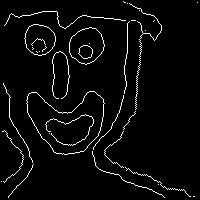
Example: image colors.jpg converted to graylevel using


>> Im = imread('colors.jpg','jpg');
>> Im = rgb2gray(Im);


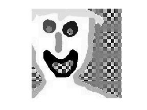
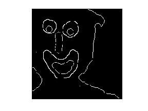
        Image Im                Roberts

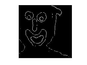
         Prewitt                  Sobel
 

Note that while they all found the most important edges,

there are breaks in the continuous edges and none found

the hairline edge or inner face edge.
 

CSE573 Fa2010 Peter Scott 04-26

---


 

The next class of edge operators looks for zero-

crossings of the second derivative (Laplacian).
 

Expanding,

  = g(i,j)-2g(i-1,j)+g(i-2,j)+g(i,j)-2g(i,j-1)+g(i,j-2)
 

which corresponds to the convolution mask   0  0 +1
                                            0  0 -2
                                           +1 -2 +2

where the pixel being recalculated (pixel (i,j) in


the equation above) is the lower right hand corner pixel


of the mask, ie. the mask origin is (3,3).



Problem with applying this mask directly, or any other

mask approximating the Laplacian operator, is that

differentiation enhances noise.
 

CSE573 Fa2010 Peter Scott 04-27

---


 

Eg:   ...................             ...................
      ...................     ...................
      .. 0  0  0  0  0  0     .. 0  0  0  0  0  0
      .. 0  0  0  0  0  0     .. 0  0  0  0  0  0
      .. 0  0  1  0  0  0     .. 0  0 +2 -2 +1  0
      .. 0  0  0  0  0  0     .. 0  0 -2  0  0  0
      .. 0  0  0  1  0  0     .. 0  0 +1 +2 -2 +1
      .. 0  0  0  0  0  0              .. 0  0  0 -2  0  0

          LRHC of image       After Lap convolution



A small amount of noise in the original image has


created a considerably larger amount after the Laplacian


filter mask has been applied. How to minimize this?


The trick is to first smooth out the noise before est-

imating the Laplacian. Usually, that is done by Gaussian


smoothing resulting in the Laplacian of Gaussian LoG:







CSE573 Fa2010 Peter Scott 04-28

---


For typical values of sigma, the mask size for the LoG

mask can be high, thus the LoG operation slow and

heavily bordered. It can be shown that the LoG operator

can be well approximated by a Difference of Gaussians

(DoG), where the variances are distinct.
 

        Difference of Gaussians (DoG):


CSE573 Fa2010 Peter Scott 04-28

---


 

In using a zero-crossing method, a final step is to

locate the detected zero-crossings in the filtered image.

Let (i,j) be designated a zero-crossing if a 2x2 mask

with its origin at (i,j) has filtered image values of


both signs in it.


To make identification more robust, can add requirement

that the absolute values exceed a threshold. Or even

better, that magnitude of the gradient (computed

independently) at (i,j) exceed a threshold.
 
 

CSE573 Fa2010 Peter Scott 04-29

---


 

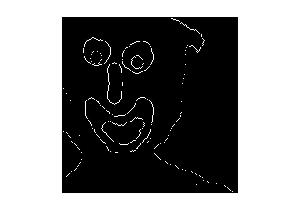
Canny edge detector
 

This method is generally considered the most powerful

of the available edge detectors. Using ideas from

signal detection theory, for a given mask origin

(i,j) first step is to find the best ms edge model,


i.e. perform optimal combined edge detection and


localization in the mean-square sense (minimum of


sum-squared errors) using an ideal edge model.


In 1-D, this looks like:

In 2-D we can fit an edge of any amplitude |f2-f1|


and any angle within the mask.


    Eg.:











If an edge is declared to have been found (|f2-f1| is

large enough) this step declares (i,j) to be an edge

pixel and returns a goodness of fit (confidence) measure



SNR = |f2-f1|/sqrt(mserror)



"Large enough" can be defined either by a numeric


treshold on |f2-f1|, or better, by a numeric threshold


on the SNR.


CSE573 Fa2010 Peter Scott 04-30

---


 

Second step is to bind together or eliminate small


broken edges. This is done with the help of two thresholds,


a high one th and low one tl. If (i,j) is not connected to


a "strong edge pixel" (m,n), one such that SNR(m,n)>th,


then apply t_h to (i,j), otherwise apply t_l.
 

Eg: Note that hairline and interior face edges ok.
 
 








CSE573 Fa2010 Peter Scott 04-31

---

 

Other edge detectors are briefly described in the

text, parametric edge models and multispectral

edge detectors. Please read all assigned material,

in class we will only discuss the more important

material.
 
 

CSE573 Fa2010 Peter Scott 04-32

---


 

Line detectors
 

In some images lines as opposed to edges are

important. A line is a long thin connected region

whose crossectional width is constant.
 

If we assume the lines to be white lines one pixel

wide, we can use a compass set of masks like
 

0  0  0  0  0     0  0  0  0  0
0 -1  2 -1  0     0  0 -1  2  1
0 -1  2 -1  0 ,   0 -1  2 -1  0  , etc.
0 -1  2 -1  0    -1  2 -1  0  0
0  0  0  0  0     0  0  0  0  0
 

Each one is a matched filter which is matched to a

line segment of specific length oriented in a specific


direction. A matched filter is a mask identical to an


object we seek, when it is over that object the filter


output will be high.
 

CSE573 Fa2010 Peter Scott 04-33

---


 

Dynamic mask selection schemes
 

All methods discussed so far assume that the

mask size and shape are selected in advance and

not varied as the mask moves across the image.

Better performace can often be had by varying

the mask depending on the data under it. The

price is higher complexity, slower execution.
 

  Adaptive smoothing: for each pixel (i,j),

  build a region outward by connected pixels

  as long as |f(k,l)-f(i,j)|<=T1. Then apply

  a smoothing filter with that as its mask.
 

  Adaptive histogram equalization: as above,

  build homogeneous regions. Then do histogram

  equalization separately on each region.
 
 
 

CSE573 Fa2010 Peter Scott 04-34

---


 
 

Eg:



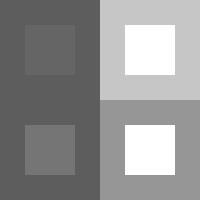
                     Original          Histogram-equalized
 
 





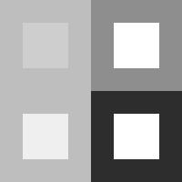
                  Adaptive Histogram-equalized
 
 

CSE573 Fa2010 Peter Scott 04-35

---


 

Other dynamic mask selection schemes such as contrast

enhancement are described in the text. Adaptive equal-

ization and smooting are the most important, though.
 

Final note: you are not responsible for Section 4.4

on image restoration techniques.
 
 

CSE573 Fa2010 Peter Scott 04-36

---