CSE668 Lecture
Slides Spring 2011
8. Passive Motion Analysis
Required
reading:
Trucco and Verri,
"Introductory
Techniques for 3-D Computer Vision," Chapter 8.
We conclude study of passive vision for 3-D and motion
recovery by considering 3-D computer vision problems
in which there is relative motion between the camera
(or cameras) and objects in the scene, and multiple
images
with
at least some overlap of the fields of view.
Eg: Sequence of video frames taken with fixed camera
model,
several
objects
moving
in
the
scene.
Eg: Capture an image of a still object, change the
extrinsic
camera
model,
take
a
second
image.
The
relative
motion might be due to either egomotion or
independent
object motion.
Note that stereo imaging can be considered a special
case of motion analysis for still objects (take one
image,
move
camera, take second image).
CSE668 Sp2011 Peter Scott 05-01
Motion
analysis is important for two quite different
reasons:
1. In both natural and computer vision, objects
we need to recognize and characterize are
often in motion, so we need to be able to
do
shape
modelling
and
OR
in spite of motion.
Eg: Read a
street sign as we drive past it quickly.
Eg: A juggler
needs to catch a tumbling bowling pin by
its
neck.
2. Visual cues due to motion can be very helpful
deriving important information about the scene
semantics, the meaning of the scene. There are
things
we
can
work
our
because of motion.
Eg: We walk
around a statue to appreciate its full 3-D shape.
Eg:
Random
dot sequence imagery.
CSE668 Sp2011 Peter Scott 05-02
Eg: Time-to-impact can be computed from the rate of
change of the size of an object.
Assume black dot is moving with velocity v
parallel to the z axis and z(to)=Do. We want
to determine the time-to-impact t'(t) such that
z(t'(t))=0. Clearly t'=(Do-vt)/v, but we only
know
l(t),
the
image
location
of
the dot.
CSE668 Sp2011 Peter Scott 05-03
But
l(t)
=
L*f/[f+(Do-vt)]
=
L*f*(f+Do-vt)-1
dl/dt = -L*f*(f+Do-vt)-2*(-v)
=
l(t)*(v/[f+Do-vt])
For
Do>>f
l(t)/(dl/dt)
=
(Do-vt)/v
=
t'(t)
So just from the image location at any time t, and its
rate of change at that time, we can determine the time
to impact t' (in practical situations, estimate t').
There
is of
course no way to get t' from a still.
CSE668 Sp2011 Peter Scott 05-04
The basic problem of motion analysis is to derive
scene semantics from high frame rate image sequences.
That is, for much of this work we will assume the
displacement of a typical object point between
successive
images is small.
The assumption of incremental displacement makes the
correspondence problem much easier than in stereo,
where
the
disparity can be large.
Using the assumption of incremental displacement, we can
make the approximation that the brightness value of a
typical image point does not change between successive
frames. Thus the correspondence problem becomes that of
estimating the apparent motion of the image brightness
distribution,
what is called optical
flow.
CSE668 Sp2011 Peter Scott 05-05
Optical
flow
Let E(x,y,t) represent the image brightness at point
(x,y)
in image coordinates at
time t. An image point
(x,y)
will appear at the
point
x+dx, y+dy, at time t+dt
if
it has velocity vector, which we refer to as the
motion field
vector v
v(x,y,t) = [∂x/∂t, ∂y/∂t]T
Over
an infinitesimal increment of time and space we assume
the
brightness of that same object point will not
change,
ie.
E(x+dx,y+dy,t+dt) = E(x,y,t), or dE(x,y,t)=0.
CSE668 Sp2011 Peter Scott 05-06
But
dE
=
∂E/∂x dx + ∂E/∂y dy + ∂E/∂t
dt
and for dx = ∂x/∂t dt, dy = ∂y/∂t dt, where
[∂x/∂t ∂y/∂t]T is the motion field (velocity vector) v,
we can write the basic equation of optical flow, the
Image
Brightness Constancy Equation (IBCE)
vx ∂E/∂x + vy
∂E/∂y + ∂E/∂t
= 0
where vx = ∂x/∂t, and vy = ∂y/∂t, the x and y components
of the motion field, defined as the velocity with which
fixed points in the scene move across the image plane.
The motion field does not in general correspond to
the true 3D motion of scene points. They correspond
only in the case where an object point is moving only
in the plane perpendicular to the optical axis (no depth
movement or
rotational movement out of that plane).
CSE668 Sp2011 Peter Scott 05-07
Typically,
the
image
brightness
partials
∂E/∂x, ∂E/∂y
and ∂E/∂t are estimated from the image sequence and
plugged into this equation to get the motion field.
Eg: Brightness values in the same image region in
two successive frames IM(i,j,k), IM(i,j,k+1) are:
...10
16
12...
...10 15 12...
...12 14 11...
...13 15 14...
...15 14 10...
...17 14 12...
IM(i,j,k) IM(i,j,k+1)
Using first forward difference approximation to
estimate the partials,
for the pixel at the center
of this region at time k,
∂E/∂x ≅ IM(i,j+1,k)-IM(i,j,k)
=11-14 =
-3
∂E/∂y ≅ IM(i-1,j,k)-IM(i,j,k)
=16-14
= +2
∂E/∂t ≅ IM(i,j,k)
-IM(i,j,k+1)=15-14 = +1
So
-3vx + 2vy + 1 = 0 by IBCE
CSE668 Sp2011 Peter Scott 05-07a
But
there is an
obvious problem in using the IBCE to get
vx
and
vy, the
x and y
components of the motion field: for
a given point
(x,y,t) in the sequence, this constitutes just
one equation
in
two unknowns vx
and
vy.
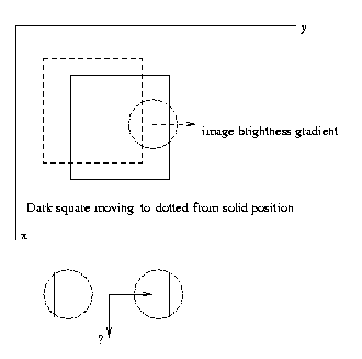
Let [vx vy]T be the actual motion field and [vx' vy']T
be any vector orthogonal to the image brightness gradient
[∂E/∂x ∂E/∂y]T. Then we can add any amount of the
orthogonal vector to a solution of the image brightness
constancy
equation and still have a solution, since
([vx vy] + a [vx' vy'])T[∂E/∂x ∂E/∂y] + ∂E/∂t = 0
Thus,
from the IBCE we can
only determine the component
of the motion
field
in the
direction of the spatial
image gradient. The
component of the motion field in the
direction
orthogonal to the image gradient direction is
not revealed by
solving the IBCE.
Eg
CSE668 Sp2011 Peter Scott 05-08
Solving
the image brightness equation
Our plan is to gather an image database E(x,y,t),
compute the partials of brightness E, and use the IBCE
vx∂E/∂x + vy ∂E/∂y +∂E/∂t= 0
to
approximate the normal component of the motion field
v(x,y) at each
t. We will designate the normal component as
the 2-D vector
v'.
As
noted earlier,
the normal component of v is parallel
to the image
gradient ∇E =
[∂E/∂x ∂E/∂y]T. So we can
write
v' as
v' = vn (∇E)/||∇E||
where ||*|| denotes
the Euclidean
norm. Here vn is a non-
negative scalar
that indicates the length
of
the normal
component
vector v', which points in
the ∇E
direction.
∇E/||∇E|| is the unit
vector pointing in the
direction of
the image
gradient ∇E.
CSE668 Sp2011 Peter Scott 05-09
Plugging
v'
into
the
IBCE,
vn (∇E)T(∇E)/||∇E|| + Et = 0
or vn = - Et/||∇E||
We can compute the normal component easily once we
have the image spatial brightness gradient ∇E,
and
the
temporal brightness derivative Et. Substituting vn
back, the final
expression for the normal component v' is
v'= vn (∇E)/||∇E||= - Et(∇E)/||∇E||2
Eg: At a given (x,y,t) ∇E=[2 -1]T and Et=3. Then
vn=-3/sqrt(5) and v'=[-6/5 3/5]T.
It is important
to keep in mind that v' is only part of
the desired
motion field, the part normal to the image
gradient ∇E at (x,y,t).
There is
in general a second
component,
which is perpendicular to the image gradient
∇E, which the IBCE
cannot help to determine.
Sometimes the normal component is all you need. For
instance,
in
the case of purely translational motion in
the (x,y) plane, the motion field vectors of a rigid body
are all equal, and this can be used to determine the
motion
field
from its normal component.
CSE668 Sp2011 Peter Scott 05-10
Eg: x-y plane translational motion of a rigid body:
Since
the
body
is rigid and undergoing pure translational
x-y motion, all motion field vectors must be
identical. So
the motion field at each point can be
determined by combining
the normal component there with the normal
component determined
elsewhere at any point where the image
gradient is orthogonal
to its value at the given point.
But
in more
general cases, we need to approximate the
complete motion field, not just the normal component.
We will refer to an approximation of the motion field
based on image brightness partials as an optical flow
field.
CSE668 Sp2011 Peter Scott 05-11
Before
developing
methods
for
computing
optical
flow,
it should be noted that the true motion field v
does not exactly satisfy the IBCE, even in the simplest
case. It is shown in Trucco, for instance, that for
Lambertian surfaces and a single point source of
illumination
infinitely far away,
vx∂E/∂x + vy ∂E/∂y + Et = ρ IT(ωxn)
where ρ is the albedo, I the illumination vector,
ω (omega) is the angular velocity vector, n the
surface
normal, and x the vector product (8.21 p 194).
So
even in this simplest of cases, only if the object
motion
is pure translational (ω=0) will the
IBCE be
correct.
CSE668 Sp2011 Peter Scott 05-11a
While only an approximation, the
optical
flow field
that
satifies the IBCE often is, however,
a useful
approximation to the motion field. This is often true
even in more complex cases such as multiple local
illumination
sources, projective projection geometry,
non-rigid
body motion and modest amounts of rotation.
Much
work has gone into the design of optical flow
algorithms
that use the information about the motion
field
it contains while minimizing the errors that come
from
the fact that optical flow is, at best, an approximation
to
the desired quantity, the motion field.
CSE668 Sp2011 Peter Scott 05-12
The
constant flow algorithm
For rigid body motion, we may assume that over most
small visible surface patches the motion field v is
constant. This is exact if the rigid body is undergoing
purely
translational motion in the x-y plane, otherwise
it's only true
to a good approximation.
By
writing the IBCE at each of nxn set of pixels
in a small patch, we can change one equation in two
unknowns to n2 equations in two unknowns and solve
the
now
over-defined system by least squares. That is
the core idea
of the constant flow algorithm.
CSE668 Sp2011 Peter Scott 05-13
Writing
the
IBCE
at
pixels
p1..pN
on
a
small patch,
and
assuming
v is constant over the patch (this is
called the constant flow assumption), let E(p)
be
the
brightness at pixel location p and time t:
∇E(p1)Tv + Et(p1 ) =0
∇E(p2)Tv + Et(p2) =0
...
∇E(pn2)Tv + Et(pn2)
=0
or Av-b=0
where A is n2x2, b is n2x1 and v is the common 2x1
unknown motion field for all pixels on this patch.
Then
ATAv-ATb=0
and we have an unique least squares solution
v'(p) = (ATA)-1A Tb
Note that v is the true unknown motion field and
v' the optical flow field. They will be exactly
equal only in the case where the image partials are
known exactly without error or noise.
CSE668 Sp2011 Peter Scott 05-14
Eg: From
Barron, J.L. et. al., "Performance of Optical
Flow Techniques," IJCV, 12:1, 43-77, 1994.
Notice that the motion vector estimates in regions of high local contrast such as the rim of the round table on which the Rubik's
Cube sits are quite accurate while other regions, like the top of
that table, are very poorly estimated.
CSE668 Sp2011 Peter Scott 05-14a
The
most common
version of the constant flow algorithm uses
a square mask
centered about the point p. One project idea
might be to used censored averaging of some kind to avoid
using points on both sides of a rigid body bounding edge.
Eg: Object undergoing (x,y,z) translation against a
moving background. Averaging in the indicated
circle
would
yield
bad
estimates.
CSE668 Sp2011 Peter Scott 05-14b
Note
that since calculations are done patch by patch
independently,the
constant
flow
algorithm
does
not
actually
require
the entire object to be a rigid body undergoing
pure
translational motion, just that each patch be. Of
course,
if the object is not rigid undergoing pure translation,
there
will be formal contradictions between the treatment of
overlapping
patches. Thus we should say that constant flow
is
an approximation to the motion field based on the
assumption
of local rigid translation rather than global rigid
translation.
CSE668 Sp2011 Peter Scott 05-15
The
feature
tracking
method
The constant flow algorithm, a differential
calculation, gives you a dense optical flow field
output (one motion estimate per pixel) but is clearly
going
to be
noisy, for two main reasons:
1. The estimation of ∇E(p) and Et(p) from E
will be noisy;
2. The IBCE is never exactly satisfied.
CSE668 Sp2011 Peter Scott 05-16
An
alternative is the feature tracking class of
algorithms, which have opposite characteristics: they
output only a sparse optical flow, but (for well
designed algorithms) the flow estimate is much less
noisy. These algorithms rely on solving the
correspondence problem (computing disparity) for
prominent features. Disparity per unit time is a direct
approximation to the desired motion field.
CSE668 Sp2011 Peter Scott 05-17
Structure
from
motion
Given a (sparse or dense) optical flow field, can we
determine the structure of the rigid body being
imaged? By structure we mean the 3-D coordinates of
a
set of
surface pixels of the object.
1.
From a
sparse optical flow field:
Given a sparse optical flow field from a single object
assumed to be moving as a rigid body and viewed in
orthographic projection, we may use the following
algorithm to compute both structure (the 3-D locations
of each pixel in the sparse set), and the motion
parameters of the object: its translation and
rotation vectors. So this algorithm should really
be called "motion and structure from sparse optical
flow."
CSE668 Sp2011 Peter Scott 05-18
Let
pij=[xij
yij]T, i=1..N frames, j=1..n pixels
be the set of pixels with known disparties. Begin
by computing the centroid pi for each frame by
averaging
the n pixels pij.
The motion of a 3-D rigid body is governed by
v = -T - ωxp
where T is the translation and ω the rotation vector,
x is vector product, and v is the velocity vector at
location
p
(v, T, w and p are all 3-D vectors). The
vector product
is computed by the "right-hand-rule"
to be
ωxp = [ωypz-ωzpy
ωzpx-ωxpz
ωxpy-ωypx]T
First consider translation T. The x and y components
are just the disparity rates
[Txi Tyi]T = Ti = (pi+1-pi)/(ti+1-t i)
The z component of T cannot be computed, as we are
assuming
orthographic projection.
CSE668 Sp2011 Peter Scott 05-19
Eg: A point undergoing only z-translation will not
move in orthographic projection. Two points
with identical T and ω vectors except for Tz
will,
by
superposition,
move
identically.
Now to get the rotation and shape parameters, define
the
central
or registered coordinates x~ij, y~ij
[x~ij y~ij]T = [xij yij]T - pi for i=1..N, j=1..n
Then with X~ and Y~ the x~ij and y~ ij matrices, define
the
registered measurement matrix W~
W~ = [X~T Y~T ]T
CSE668 Sp2011 Peter Scott 05-20
It
turns out
(see Trucco 203-208) that W~ can be
factorized as a product of just what we want: a
rotation
matrix R and a structure matrix S
W~ = RS
where
R
=
[i1 ... iN j1 ... jN]T
and the rotation of frame k is specified by the
orthogonal axes (ik, jk, ikxjk )
and
S = [P1 ... Pn]
where P1 is a vector in R3 correponding to the
intial position at t=t1 of the point {p1j, j=1..N},
2. From a dense optical flow field: select a set of n
points, correspond them over the N frames, and proceed as
above.
CSE668 Sp2011 Peter Scott 05-21