CSE668
Principles of Animate Vision Spring 2011
6. Vision for navigation
In
this section of the course we will consider the "motion
competencies," those animate vision skills associated with
relative motion between the camera and objects in the
scene.
Motion
competencies
include:
* egomotion estimation
* obstacle avoidance
* visual servoing
* tracking
*
homing
With only about two weeks to discuss all the motion
competencies, we cannot go into much depth but rather
we will take a representative approach to each of these
problems
and
read
the
paper
and
describe
the
method.
CSE668 Sp2011 Peter Scott 08-01
Egomotion
estimation
In the Fermuller-Aloimonos heirarcy, motion competencies
are the most basic and among them, egomotion estimation
comes first. There is good reason for both of these
choices.
Motion competencies are the most basic, they argue, because
they are the simplest and most primitive in natural vision.
Recall that the snail has a single photodetector and senses
changes
in
brightness
as
possible
shadow
of
a
predator
looming.
Egomotion estimation comes first because it is necessary
to separate egomotion from independent motion of objects
in
the
scene
in
order
to
do
any
other
motion
competency.
Eg: Cannot effectively avoid an obstacle unless you know
if
it
is
approaching
you,
or
you
approaching
it.
Eg: Cannot devise a good homing stategy on a moving
object unless you know how it is moving.
CSE668 Sp2011 Peter Scott 08-02
One way to do egomotion estimation is to determine
the 3-D locations of several stationary feature
points in an image sequence and then apply the
Structure-from-motion Theorem (Sonka p. 510).
With as little as three projections of four points,
we can recover both the 3-D rigid displacement
vectors (shape) and the motion parameters, the
translation and rotation vectors. Since the points
are stationary, the camera motion will be the
negative
of
the
perceived
object
motion.
Problems: need a calibrated camera, must solve the
correspondence problem for each feature point, and
must
be
sure
that
the
feature
points
are
stationary.
Eg: You are sitting on a train in the station and the
train next to you starts to glide slowly backward.
Are
you
moving
forward
or
it
moving
backward?
CSE668 Sp2011 Peter Scott 08-03
In contrast, active vision approaches do not recover the
3-D structure of the scene in order to determine egomotion.
They are based on the apparent motion field created as the
camera moves about while fixating on scene points. Apparent
motion of a point in an image sequence is the motion of
that
point
measured
in
image
coordinates.
Eg: If you are fixated on an scene point right along
your egomotion translational velocity vector, and
you are not rotating the camera as you move, the
apparent motion field is purely radial.
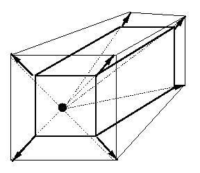
So, if you can produce radial optical flow, then the
egomotion must be pure translational along the optical
axis of the system, which points directly at the
focus of expansion (FOE).If you are moving away from
the object, the FOE becomes the focus of contraction
(vanishing point).
CSE668 Sp2011 Peter Scott 08-04
Using the above, its easy to estimate egomotion parameters
in world coordinates, like "I'm moving straight towards
the middle of the closest face of that rectangular object."
Note that we can't make a quantitative estimate of the
magnitude of our egomotion vector, ie. our egomotion speed,
but only its direction. We would need to know how big the
objects in our FOV are in order to determine speed as well.
Eg: Situation 1: you are a distance d from an object
O oriented with pose p and are moving directly
towards it with a velocity vector e.
Situation 2: you are a distance 2d from an object
O' which is identical to O except twice as
big, is oriented with pose p and you are moving
directly towards it with a velocity vector 2e.
You
cannot
distinguish
these
situations.
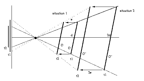
Note that in this example you cannot quantify speed, but
you can quantify time-to-collision, which is the same for
both situations. We will consider this in studying the
problem
of
obstacle
avoidance.
CSE668 Sp2011 Peter Scott 08-05
Determining apparent motion
We consider only the case of stationary objects in
which
the optical axis is aligned with the egomotion velocity
vector (i.e., you are looking where you are going).
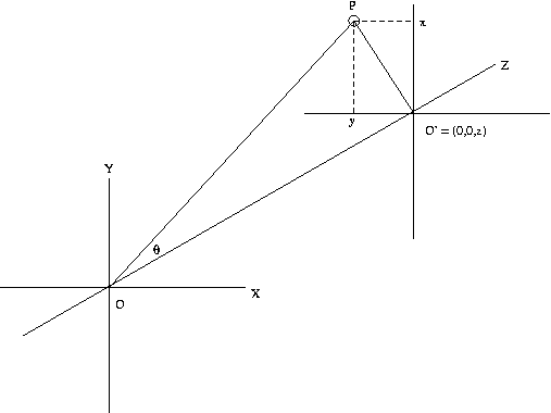
The fixation frame is the coord system shown with origin
at O', the point we are looking at, and the plane containing
O' and perpendicular to the optical axis is called the
fixation plane.
CSE668 Sp2011 Peter Scott 08-05a
Let P=(x,y,z) be a point in camera coords. Define the
view
angle θ as the
plane angle shown below in the
O-O'-P
plane.
In
this
plane,
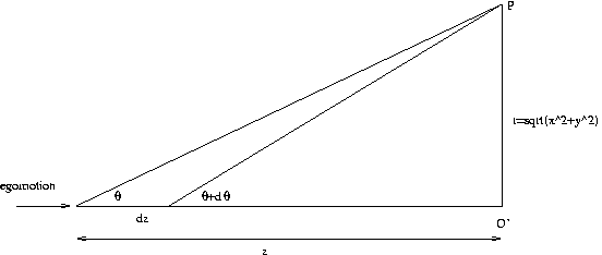
tan θ = r/z
d(tan θ) = dθ/(cos2 θ)
d(r/z) = -r/z2 dz = -tan θ/z dz
Then
dθ/dz = (cos2 θ)(-tan θ/z)
= (-cos θ)(sin θ)/z = -sin(2θ)/(2z)
CSE668 Sp2011 Peter Scott 08-05b
Let the egomotion speed be s = -dz/dt. Then
dθ/dz = -dθ/(s dt) and
dθ/dt = (s/(2z))(sin(2θ))
This tells us how fast the view angle θ of a point
will be
changing
as
we
move
in
the
direction
we
are
looking.
Note
that
it
depends
on
the
ratio
s/z,
and
on
the
view angle θ itself.
CSE668 Sp2011 Peter Scott 08-05c
Eg: The image of a stick (camera coords of endpoints
shown) which we see while walking with speed 1 m/s is
(units: m)
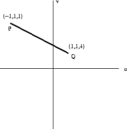
For P, θ = arc tan sqrt(x2+y2) = .955 rad.
dθ/dt = (s/2z)(sin 1.91)= .472 rad/sec
For Q, θ = arc tan sqrt(x2+y2) = .340 rad.
dθ/dt = (s/2z)(sin 0.68)= 0.08 rad/sec
CSE668 Sp2011 Peter Scott 08-05d
So after a short period of time, the image will be
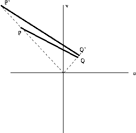
The
apparent
motion
of
P
in
the
image
plane
will
be
.472/.08,
or
about
6
timesthat
of
Q.
Why
is
this?
P
is
closer
to
the
camera,
so
its
apparent
motion
will
be greater.
CSE668 Sp2011 Peter Scott 08-05e
View
angle
and
(u,v)
For uo=vo=0, there is a simple
proportionality between
the radius of a point in the z-plane and the radius on
the image plane:

By
similar triangles, rz/ri = z/f or ri =
(f/z) rz.
If in addition there is no skew (intrinsic parameter
b=0)
then the image coordinates are related to the camera
coordinates by the linear relationship
(u,v) = (f/z)
(x,y)
CSE668 Sp2011 Peter Scott 08-05f
The relationship between ri and θ is gained by noting
that tan θ = rz/z, so
ri = f tan θ, θ = arc tan ri/f
dri/dt = f (1/cos2 θ)(s/2z)(2sin θ*cos θ)
= (s f tan θ)/z
The apparent
radial motion of an image point is proportional
to the egomotion velocity s and to the tangent of
the
view
angle θ. This
of course assumes the fixation point is
stationary in world coords, and you are looking
where you
are going (optical axis and egomotion velocity
vector are
collinear).
Eg: For uo=vo=b=0, f=50mm, what is the image radius
ri
and view angle of the scene point (x,y,z) =
(100,10,3000)
(units:mm).
(u,v)=(f/z)(x,y)=
(50/3000)(100,10)=(1.67mm,.17mm)
ri = sqrt(1.67^2+.17^2) = 1.68mm
θ = arc tan 1.68/50 = .0336 rad
= 2o.
CSE668 Sp2011 Peter Scott 08-05g
The
Barth-Tsuji
algorithm
Required
reading:
Barth and Tsuji, Egomotion
determination through an intelligent gaze control strategy, IEEE Trans
Systems, Man and Cybernetics, v 23 (1993), 1424-1432.
This algorithm
for estimating egomotion is based on the
previously
stated
idea
that
assuming
pure
translation,
there
is
no
apparent
motion
along the optical axis when
the
optical
axis
is aligned with the translational
velocity
vector. There is no
radial motion because the
tangent
of
the
view
angle
is
zero,
and
no
other
motion
because
all
apparent
motion
is
radial
in
this
case.
CSE668 Sp2011 Peter Scott 08-05h
Barth
and
Tsuji
assume
there
is
a
single
mobile camera
The algorithm proceeds by specifying a sequence of
sudden changes of the optical axis of the system,
called saccades, which are designed to bring the optical
axis into alignment with the translational velocity
vector.
Once
they
are
in
alignment,
then
* translational egomotion velocity vector is aligned
with the optical axis and thus its direction is
known;
* rotational egomotion velocity vector is the negative
of
the
apparent
motion
along
the
optical
axis.
The latter follows from the fact that since there is no
translational component, all motion at the FOE must be
due
to
rotational
movement
of
the
camera.
CSE Sp2011 Peter Scott 08-06
The logic of the saccade calculation is split into
two parts: first consider which direction to saccade
in, then how large a saccade to make in that direction.
1.
Saccade
direction:
Suppose at time t you are maintaining fixation at the
scene point Z. Assume that close (in image coordinates)
to Z there are scene points which are at different
distances
to
the
camera
than
Z.
Then
in
order
to
move
towards
alignment
of
the
optical
axis
with
the
velocity
vector,
you must saccade in the opposite
direction of
apparent motion
of the scene points which are
closer to
the camera than Z.
CSE Sp2011 Peter Scott 08-07
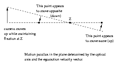
How do we know which points are closer? Remember from our
previous discussion of motion parallax that points behind
the fixation point move in the same direction as the
egomotion translation producing the motion parallax, points
in front move in the opposite direction.
CSE Sp2011 Peter Scott 08-08
Why does saccading in opposite direction of close
points work?

One way to recognize the closer points, F+, is to
note that during the maneuver the camera head must
rotate either cw or ccw to maintain fixation at Z.
Points that appear to rotate in the same direction
are
called
F+
and
opposite,
F-.
Another, if camera head rotation is not known, is to
note that average velocity in F+ is higher (equal
displacement of a point nearer the camera results
in greater displacement on the image plane). This
works as long as the points in F+, F- are equally
distributed around the fixation point, or can be
guaranteed if a single point in F+ is closer than
half the distance to the fixation point.
CSE Sp2011 Peter Scott 08-09
2.
Saccade
magnitude:
How
much
do
you rotate? In the paper, it is shown that
if
you
use
the
iterative
rule
delta(θ)
=
-K(|F+|-|F-|)
where F+ is the average apparent motion of the set of
points near the fixation point in image space which
are moving in the same direction as the camera is
rotating in order to maintain fixation on Z, and F-
the average for the the opposite, then for small
displacements along the velocity vector, this is
well-approximated
by
delta(θ)
~
-K' sin(θ)
which converges to zero for suitable choice of K'.
Here θ measures the angle between optical axis and
velocity
vector.
CSE Sp2011 Peter Scott 08-10
Finally, as mentioned earlier, once you have alignment
(or near-alignment) between the translational velocity
vector and the optical axis, you can determine the
yaw and pitch rotational speeds by observing the apparent
rotational
velocity
of
points
along
the
optical
axis.
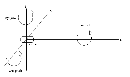
Yaw is rotation about the vertical axis, roll is rotation
about the optical axis, and pitch about the other
horiontal axis
CSE Sp2011 Peter Scott 08-11
Eg: Suppose that at t, we have alignment and are fixated
to a point on the optical axis. As the camera
moves in yaw (rotation about the y axis) and pitch
(rotation about the x axis) to maintain fixation, the
negative of these angular rates of change are the
rotational velocities in these directions. Note that the
rotational velocity in the roll direction (rotation about
the optical axis) cannot be determined. However, this can
be easily determined from the apparent tangential motion
of
all
other
points.
CSE Sp2011 Peter Scott 08-12
Note how natural this animate vision algorithm is. We
seek to look in the direction we are moving. We get
clues for where to saccade next by a sequence of fixations
during which we observe the motion parallax. Once we
are looking where we are going, we both know where we
are going (translational motion) and how our head is
twisting (rotational motion) from the view along the
foveal
axis.
CSE Sp2011 Peter Scott 08-13
As a final note, lets measure the Barth-Tsuji scheme
against the active vision and animate vision paradigms.
How
would
it
score?
Active vision:
* Vision is not recovery.
* Vision is active, ie. current camera model selected
in light of current state and goals.
* Vision is embodied and goal-directed.
*
Representations
and
algorithms
minimal
for
task
Animate vision: Anthropomorphic features emphasized, incl.
* Binocularity
* Fovea
* Gaze control
*
Use
fixation
frames
and
indexical
reference
CSE668 Sp2011 Peter Scott 08-14
Collision avoidance
Required
reading:
Kundur and Raviv, Active vision-based
control schemes for autonomous navigation tasks, Pattern Recognition v
33 (2000), 295-308.
If the camera platform (robot, vehicle, etc.) is to move
in the real world of objects which are also moving, and
of stationary objects whose locations are not mapped in
advance, we must detect collision threats and react to
them.
This
behavior
is
called
collision
avoidance. An
equivalent
term
is
obstable
avoidance. We will use the
former
term,
as
do
Kundur
and
Raviv
(KR).
The recovery-based approach to collision avoidance would
be to recover the relative shape and motion parameters of
each object suface in the FOV and determine which, if any,
will collide with the camera platform or pass too close
to it for comfort. Then revise egomotion parameters to
protect
against
collision
while
maintaining
task
awareness.
CSE668 Sp2011 Peter Scott 08-15
The problem with this approach is that the representations
and algorithms are vastly over-complicated for the task.
We don't have to recover an accurate shape model and pose
and translational and rotational components of motion of
the person we are about to pass in the hallway, we just
have
to
make
sure
we
are
out
of
his
way
as
we pass.
Details of shape and motion of threat objects are
irrelevant once they have been recognized as threat
objects and coarse estimates of their time-to-collision
have been made. For non-threat objects, shape and motion
are
of
no
consequence
(in
the
context
of
collision
avoidance).
CSE668 Sp2011 Peter Scott 08-16
Recognizing
threats
How do we accomplish obstacle avoidance when we are out
walking? We are constantly on the lookout for objects
that are pretty near to us and which we are approaching,
these represent threats. Once identified, each threat
can be given our attention, from the most threatening
on
down.
Consider
a
threat
map, which is a
mapping from (u,v),
the current image, into R1, the degree of collision threat
associated with each pixel. How could we determine such
a useful map? One way would be to estimate the time-
to-collision tc with each visible object surface patch.
Then the inverse of tc could be the threat metric.
CSE668 Sp2011 Peter Scott 08-17
Threat
map
construction
for
stationary
scenes
In case that the only scene motion is due to egomotion,
this
paper
shows
a
strategy
which
starts
from
"looking
where
we
are
going"
and
ends
with
the
computation
of
time-to-collision
tc for
each object pixel in the scene.
Thus
we
get
the
threat
map
in
a
straightforward
fashion,
and
the
threat
map
is
all
you
need
for
collision
avoidance.
CSE668 Sp2011 Peter Scott 08-17a
Note
that
"looking
where
you
are
going"
is the output
of
the
algorithm
described
by
Barth
and
Tsuji.
This
"visual
behavior"
can
only
be
accomplished
if
you
have
mastered
the
motion
competency
of
qualitative
egmotion
estimation.
So
the
output
of egomotion estimation is
a
precondition
of
obstacle
avoidance. This is an example
of
Fermuller
and
Aloimonos'
concept
that
competencies
build in a sequential fashion.
CSE668 Sp2011 Peter Scott 08-18
Let O be an object point in the scene. Consider the plane
containing O and the optical axis z of the camera. Let
the coordinates of this plane be (r,z), where z is the
optical axis and r is the radial distance of O from
the
optical
axis.
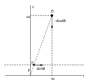
By
similar
triangles,
f/ri = zo/ro, ri = f ro/zo
dri/dt
=
d/dt
(f ro/zo) = (-f ro/zo2) dzo/dt
Substituting
in
ri,
dri/dt
=
(ri)(-dzo/dt)/zo
CSE668 Sp2011 Peter Scott 08-19
Now if the egomotion velocity dzo/dt, assumed to lie
along the optical axis, is maintained, the point O
will
collide
with
the
z=0
zero-depth
plane
at
time
tc = zo/(-dzo/dt)
Thus the time-to-collision tc for O can be computed from
the
optical
flow
at
O's
image
point
ri as
tc = ri/(dri/dt)
Now if we take the inverse of tc to be the threat metric,
we can compute the threat map pixel by pixel using the
radial
optical
flow dri/dt,
1/tc
=
(dri/dt)/ri
Thus we can do obstacle avoidance in a stationary scene
by "worrying about" objects or surface patches which are
moving
rapidly
away
from
the
FOE.
Note that this can also be written
1/tc = (dri/dt)/ri = d(ln
ri)/dt
though we will not use this form in the present context.
CSE668 Sp2011 Peter Scott 08-20
Object
avoidance
based
on
the
visual
threat
cue
(VTC)
A few equations above we wrote
dri/dt = (ri)(-dzo/dt)/zo
Dividing by ri,
(dri/dt)/ri = (-dzo/dt)/zo
So
1/tc
we
computed
above
can
be
rewritten
1/tc = (-dR/dt)/R
where (changing notation to follow the KR paper)
R is the depth range of the object point. Note: ri
is the radius in the image plane at which the object
point is seen, R is the z-coordinate value of the object
point in camera coordinates.
The authors next modify this 1/tc threat
metric in
two
following
ways. First,
lets define a desired minimum
clearance
z=Ro.
This
corresponds to a "personal space" or
"no-fly
zone"
we
wish
to
maintain
in
front of the camera
coorinate
origin
to
keep
the
camera
platform
safe from
an
unexpected
maneuver.
Then
the
time
at
which
the
object
will
penetrate
this
zone
is
to
=
(R-Ro)/(-dR/dt)
So to is the time-to-mininum-clearance.
CSE668 Sp2011 Peter Scott 08-21
Second,
lets scale the resultaing threat metric
1/to
=
(-dR/dt)/(R-Ro)
by
Ro/R,
which
measures
how
close
the
threat
object
is
to
the desired minimum clearance. Time-to-minimum-clearance
to assumes that the object will continue on its current
course. But if it is close, it might speed up or head
right at us, so we should take its proximity into
account also. Combining the time-to-minimum-clearance
threat factor and the proximity-threat factor, we get
the
Kundur-Raviv
(KR)
Visual
Threat
Cue
(VTC)
VTC = (Ro/R)((-dR/dt)/(R-Ro))
CSE668 Sp2011 Peter Scott 08-22
If we could construct a threat map using the VTC, we could
use it as above. But it involves the range R to the object.
If we need to compute that from the image, this is another
recovery-based
method,
not
a
true
active
vision
method.
To get around that, KR define an apparently
unrelated quantity which can be computed directly from
an
image
without
recovery,
the
Image
Quality
Metric
IQM,
is
a
mapping
from
a
specified
region
of
the
field
of
view
to
the
reals
as
follows:
IQM:
Image region Rho -> Real number
1. define an image region Rho;
2. define a window W;
3. for each point (x,y) in Rho, sum absolute
differences in gray levels between (x,y) and all
other points in W(x,y);
4. sum the results of 3. over all (x,y) in Rho;
5.
normalize
by
the
total
number
of
terms
being
summed.
CSE668 Sp2011 Peter Scott 08-23
So
the
IQM
is
a measure of how variable the image is over
spatial scales limited to the chosen window size. This
measure
is
averaged
over
a
selected
image
region
Rho.
We
can
think
of
the
IQM
as
an
indicator
of how sharply in focus the
object
segment
surrounding
that
pixel
location
is.
KR
claim:
d(IQM)/dt
is
a
proxy
for
the
VTC.
By
a
proxy,
we
mean
it
can
be
used
to
"stand
for" the VTC,
ie.
it
is
a
reasonably
accurate
model
of
the
VTC.
Clearly,
as
an
object
gets
closer
you
can
see
its
textured
surface
better,
thus
IQM
increases.
Like
the
old
saying
goes,
"Don't
fire
until
you
can
see
the
whites
of
their
eyes."
In other papers referenced in the KR paper,
they
give
some
empirical
evidence
for
this
claim.
CSE668 Sp2011 Peter Scott 08-24
The basic action of their obstacle avoidance algorithm
is to segment out a candidate image region and measure
d(IQM)/dt with Rho = segment. Based on prior training
(fuzzy system, neural network, etc.) a control scheme
reacts
to
the
proxy
VTC
by
stopping,
moving
away,
etc.
How good an active-animate method is the KR algorithm?
That remains to be seen as they explore into more
natural environments (see paper). But other than employing
indexical reference and being active, it is suspect on all
other grounds (goal-seeking, embodied, binocular, foveal,
gaze
control).
CSE668 Sp2011 Peter Scott 08-25
Visual servoing
Required
reading:
[15]
Vassallo et al, Visual servoing and
appearance for navigation, Robotics and Autonomous Systems, v 31
(2000),
87-97.
In control theory, a servomechanism is a system including
a controlled plant with measureable outputs, a controller,
and a feedback loop between them, which controls the
plant outputs to follow a desired or reference trajectory.
Servoing is the process
of following that trajectory.
Eg:
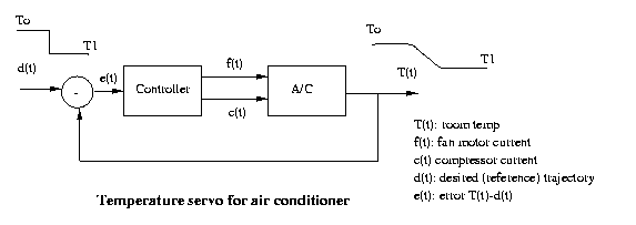
Visual servoing is the control of egomotion guided by
visual
image
sequences.
CSE668 Sp2011 Peter Scott 08-26
Examples
of
visual
servoing:
* Moving the end-effector of a robot so that
it can pick up a machine part on a coveyer belt
(robotic
hand-eye
coordination).
* Pursuit and interception of an incoming missle
by
an
anti-missle
missle.
* Guiding a welding robot to lay the weld along
a
visible
seam
between
sheet
metal
parts.
* Maintaining an autonomous vehicle in the center
of the right lane of a highway even as the road
curves
and
turns
guided
by
visual
data.
* Visual navigation along a desired path, for
instance,
following
a
corridor.
CSE668 Sp2011 Peter Scott 08-27
Visual servoing is a class of motion competencies, built
on egomotion estimation, that are essential for autonomous
movement
using
vision
sensors.
Note that visual servoing is often combined with other
visual competencies in developing useful behaviors. For
instance, we can home to a point adjacent to a conveyer
belt, then visually track a part moving along the belt,
then perform hand-eye coordination to pick it up, then
home to a parts bin, then do hand-eye to position the
hand above the bin, then release the part. Along the
way,
we
have
done
frequent
egomotion
estimation,
homing,
and
perhaps
obstacle
avoidance
as
well
as
visual
servoing.
They are the motion competencies necessary to accomplish
this
vision-supported
behavior.
CSE668 Sp2011 Peter Scott 08-28
Vassalo et al develop a nice example of visual servoing
embedded within a larger visual navigation system in
their paper "Visual servoing and appearance for
navigation" (see reading
list for full citation).
Their
task
scenario:
A
robot
must
be
programmed
to
find
and
enter
selected
offices
and
rooms
in
a
one-floor
office
space.
Design option 1: No visual servoing (no camera needed).
Memorize floorplan. Then from known initial location
and heading can compute the full sequence of control
signals to get you wherever you want to go "with your
eyes
closed."
Design option 2: Full visual servoing using a camera and
appearance-based
control. Offline
training: for each
possible
position
of
the
robot
and
orientation
of
the
optical
axis,
store
an
image.
Then
each
time
a
new
image
is
registered,
search
the
library
of
images
for
best
match.
Turn
and
move
the
robot
based
on
its
current
position,
orientation
and
the
desired
destination.
CSE668 Sp2011 Peter Scott 08-29
Neither
of
these
prove
satsifactory design options. Problems:
DO1. Small initial condition errors will produce increasing
navigational errors as you proceed. Also, cannot react
to
obstacles,
determine
closed/open
doors,
etc.
DO2. Large set of images to be stored and at each frame
input, searched for best match. So, high computational
complexity
and
large
storage
requirements.
Vassalo et al propose a compromise (DO3) in which we store
a small set of indexed landmark images. When we start
the robot, it performs a visual servoing behavior we will
call "corridor-following." As each new image comes in,
we compare it with a single image, the first landmark
image in the route. When we arrive at the first
landmark image location, we update our location
data, replace the image with the next indexed landmark
image
and
proceed.
This
is
landmark-based
navigation.
CSE668 Sp2011 Peter Scott 08-30
So DO3 combines pure visual servoing during corridor-
following with appearance-based (view-based localization)
navigation
at
a
sparse
set
of
landmarks.
The
landmark-image
matching
is
done
by
straight
image
correlation.
How
is
the
corridor-following
done?
Servoing
to
the
vanishing
point
We can follow the corridor by locating the ground plane
vanishing point and turning the robot to home in on it.
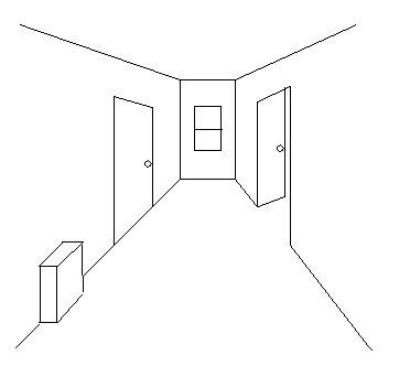
Schematic
of
an
image
of
the
corridor
CSE668 Sp2011 Peter Scott 08-31
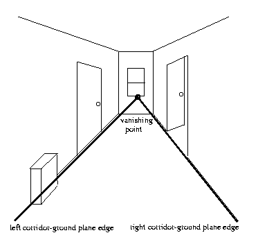
Vanishing
point
is
the
intersection of the corridor-ground plane edges.
CSE668 Sp2011 Peter Scott 08-32
To find the corridor-ground plane edges:
1. Use Sobel operators to find pixels with both
significant horizontal and vertical gradients;
2. Separate into positive and negative gradient
orientation pixel sets (left and right edges).
3. Erode with diagonal line mask to remove pixels
not on diagonal lines.
4. Find the positive and negative straight lines
with
the
largest
number
of
pixel
"hits."
CSE668 Sp2011 Peter Scott 08-33
In the paper it is shown that the horizontal image
coordinate
of
the
vanishing
point
ixv
satisfies (eqn 7)
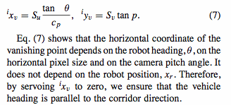
where Su is an intrinsic camera model parameter and
cp is the cosine of the pitch (downlooking angle). θ
is the deviation between the robot heading and the
direction of the corridor. So controlling ixv to zero
(centering the vanishing point in the image) is the
same as driving θ to zero (orienting the robot
to
follow
the
corridor).
CSE668 Sp2011 Peter Scott 08-34
Visual homing
Required
reading:
[16]
Nelson,
From
visual
homing
to
object
recognition,
in
Aloimonos
(ed.)
Visual
Navigation,
Lawrence Erlbaum Associates, 1997.
As was pointed out in the Vassallo paper, their scheme
combining visual servoing and landmark memory can form the
basis for visual homing, movement to a desired location
using
visual
data.
Visual homing is important in several applications
contexts:
* Robotic tool positioning
* Robotic or autonomous vehicle navigation
* Material handling
*
Object
set
manipulation,
eg.
assembly
tasks
We will study an approach to visual homing presented in
the paper by Randal Nelson, "From visual homing to object
recognition" (see above for full citation). As the
title implies, Nelson's approach has implications for
active vision approaches to the shape competencies whose
review
will
form
the
last
part
of
this
course.
CSE668 Sp2011 Peter Scott 08-35
The central questions in visual homing are: given
the
goal
(homing
to
a
specific
location),
*
What
is
my
current
state
(location
and
pose)?
* Given my current state, what motion control
actions
should
I
take?
The second question is a control engineering question
tied to the mechanics of the mobile platform and is
outside the range of this course. We will simply assume
that the motion control problem can be solved, and
concentrate our attention on using visual data for
state
determination.
CSE668 Sp2011 Peter Scott 08-36
Visual
associative
memory
State determination can be done based on visual recovery.
This passive approach is inefficient, however. Nelson
advocates the use of a pattern-recognition based procedure
called a visual associative memory. In general, an
associative memory is a memory addressed by partial
content.
Eg:
Phone number 645-23?? -> 645-2394
Eg:
Who do I know with a big nose and blond hair? That
must
be
Bob.
A visual associative memory is a store of many 2-D images,
and
given
a
new
image,
addresses
the
most
similar
image.
CSE668 Sp2011 Peter Scott 08-37
Let Ak be the kth feature of a pattern, with Ak = {ak},
where each ak is a definite value for that feature. Define
a pattern as an m-tuple P=(a1,...,am) from the pattern
space A=A1xA2x .. Am (x is Cartesian product). So a
pattern
is
a
set
of
feature
values
from
the
pattern
space.
Define a similarity function s: AxA -> R (R is the set
of real numbers) which compares patterns. There are many
such mappings which can be used as similarity functions,
for instance the norm-induced correlation similarity
measures
similarity
between
Px and Py as
s1(Px,Py)
=
||Px-Py||/sqrt(||Px||*||Py||)
where
||*||
is
a
selected
norm
over
A.
CSE668 Sp2011 Peter Scott 08-38
For his visual associative memory, Nelson uses the
similarity
measure
s(Px,Py)
=
1
-
d(Px,Py)/m
where d is the cardinality of the set of features that
are not identical, and m is the dimension of the pattern
space. d is sometimes called the "Hamming Distance."
Eg: Px = (0.384,2,green,0,to the left of);
Py
=
(0.383,2,green,0,to
the
right
of)
s(Px,Py)
=
1
-
2/5
=
3/5
So s measures the fraction of features that are identical.
Nelson selects
this similarity measure because it can be
used for categorical variables, those for which there are
only
labels
without
reequiring
any
ordering
function,
as
well
as
numerical
variables.
CSE668 Sp2011 Peter Scott 08-39
Suppose we have n patterns M={P} stored in our associative
memory. Then when presented with an input (index pattern)
Px, the associative memory's output will be the Py in M
which
best
matches
Px
max_M
s(Px,P)
=
s(Px,Py)
if
the
similarity
exceeds
a
threshold
t
s(Px,Py)
>=
t
If
the
best-match
does not exceed t we return "no match."
CSE668 Sp2011 Peter Scott 08-40
Here is how we will use an associative memory for visual
homing.
1. Store a set M of n reference patterns (camera views
mapped down to their feature values) taken at
known states (locations and poses). Label one or
more of them as goal states.
2. For each reference pattern, store the value of the
desired control action from that state.
3. For each new incoming image, map to its feature set
and pass that feature set through the associative
memory.
a. If there is a matched pattern,
perform the reference pattern control
action.
b.
If
there
is
no
match,
randomly
change
state
and go to 3.
4.
Repeat
3
until
the
goal
state
has
been
reached.
CSE668 Sp2011 Peter Scott 08-41
Eg: Want to home to a point X in front of the cubic object
with the camera optical axis perpendicular to the
closest face. Assume camera can translate horizontally
(not vertically) and rotate in yaw and pitch but not roll.
These are reasonable DOFs for a mobile ground plane robot.
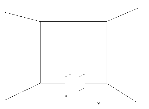
Pick a sampling grid on the ground plane and a sampling
grid in pose space (camera yaw x pitch). For each point
in this 4-D discrete state space, take a image. Define a
control action for each point as "take a step towards the
point X, and orient towards the center of any visible
object."
CSE668 Sp2011 Peter Scott 08-42
We next need to specify the visible features of this scene
that define the pattern space. There are many ways to do
this, Nelson selects a vertex feature scheme.
Here is how a binarized version of his vertex-finder
algorith works.
Divide the image space into a KvxKh grid of cells.
For a
given
image,
use
a
vertex-finder algorithm to determine
the cells in which vertices are determined to be
visible. Assign cell (i,j) to have a feature value a=1
if there is a vertex there, otherwise a=0. The pattern
corresponding
to
the
goal
state
X
will
look
like
000000000000000000000000000
000000000000000000000000000
000000000100000100000000000
000000000000000000000000000
000000000000000000000000000
000000000000000000000000000
000000000100000100000000000
000000000000000000000000000
000000000000000000000000000
If
we
are
at
a
position
like
Y,
the
index
pattern
would be
000000000000000000000000000
000000000000000000000000000
000000000001010010000000000
000000000000000000000000000
000000000000000000000000000
000010000000000010000000000
000000000001010000000000000
000000000000000000000000000
000000000000000000000000000
and, if we have a reference pattern from approximately
that same pose and location, it would have similarity 1.
The action attached to that pattern would be something
like "move one step in a direction 30 degrees ccw from
optical axis and orient the camera to the centroid of
the visible vertices."
In this example we used a binary feature space. But
in
general some or all features could be numerical.
CSE668 Sp2011 Peter Scott 08-43
In order for this scheme to work well, two conditions
should
be
satisfied:
1. Match existence condition: for each x in C, the
space of competence, there is a y in the set R
of
reference
patterns
such
that
s(Px,Py)>=t.
In
other
words,
there is at
least one match.
2. Match uniqueness condition: for all x and y,
s(Px,Py)>=t implies ||x-y||<r(x). r(x) is the
desired
accuracy
of
the
state
determination.
In
other
words,
there is at
most one match.
If these conditions are met, then we will never have
to pick a state randomly, nor confuse two states which
are far apart. If they are not met, this algorithm may
never converge. For instance if no y in R is visible
from any point we might randomly move to, we will keep
making random viewpoint changes forever.
Note that ideally both these conditions are met, but
even
if
they
are
not,
the
algorithm
may
still
converge.
CSE668 Sp2011 Peter Scott 08-44
Nelson
defines
his
vertex-finder
algorithm
as
follows.
Divide
the
image
into
a
GxG
grid.
Using
an
edge
operator,
find
the
cells
that
have
strong
edges
in
them,
and
the
dominant edge direction in each such strong-edge grid cell.
Quantize that direction into d values, eg. d=8 for
D={N,NE,E,SE,S,SW,W,NW}. Then the pattern for an image
consists in Px = (a1,a2,..,aG^2) where Ak={DU0}, U is
the
union
operator
and
0
is
the
null
edge
direction.
CSE668 Sp2011 Peter Scott 08-45
In implementing such a system, a basic design question
is how many reference patterns M must be stored in order
to satisfy the two match conditons above. By setting G
and/or t low, we can reduce card(M) and still satisfy the match
existence condition throughout C, but the lower G or t is
set, the more likely the match uniqueness condition will
be
violated
somewhere
in
C.
By setting G or t high, we are less likely to violate
the uniqueness condition but at the expense of the
cardinality
of
M.
CSE668 Sp2011 Peter Scott 08-46
Define the recognition neighborhood R(y) of a reference
pattern Py as the largest connected set of similar points
containing y (similar points are pairs (x,y) for which
s(Px,Py)>=t), ie points that would be labelled by the
same reference pattern). As long as UR(y)=C for all
reference patterns M={Py} the match existence condition
will
be
met
throughout
C.
CSE668 Sp2011 Peter Scott 08-47
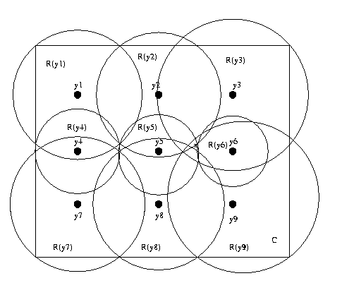
This is a 2-D example of a design satisfying the existence
condition but not the uniqueness condition. For instance,
points near x are similar to several reference points,
some of which are far apart (eg y2, y9). To satisfy
uniqueness condition, we need
||yi-yj||>r => R(yi) INT R(yj) = null.
CSE668 Sp2011 Peter Scott 08-48
In
equation
(9)
in
the
paper,
Nelson
estimates
the
spurious match probability ps in terms of the volume
in
pattern
space
of
the
recognition
neighborhood:
ps ~ pf vtot/vrn
where pf is the far-match probability (probability
that two points far apart picked randomly will match
d(x,y)>=r(x), s(Px,Py)>=t), vrn is the average volume
of a recognition neighborhood, and vtot the total
volume
of
the
domain
of
competence
C.
Roughly, vtot/vrn measures the number of far recognition
neighborhoods a point x might find a spurious match in
at
random,
and
pf
the
probability
of
a
far-match
there.
CSE668 Sp2011 Peter Scott 08-49
Eg:
Consider a building divided into N identical rooms,
and we must home into the center of one selected room
Then
pf is proportional to N, and thus so is ps.
Nelson performed some tests of his ideas using a 2-D
motion space (x-y translation, no rotation) corresponding
to "flying" above "Tinytown" with a downlooking camera.
He set G to 5, t to 0.5 and took 120 reference images
over a region of competency of roughly four "camerasfull"
of
the
Tinytown
model.
Eight
edge
directions
were
used.
CSE668 Sp2011 Peter Scott 08-50
He defined a homing action, a step direction to home
correctly (move towards the goal state) for each
reference image, and tested to see if goal states would
be
reached.
Tests were done by defining a sampling grid on C with
4x as many points as reference points, so test points
were separated by half a reference point separation.
For most tested points in C, there was a match and the
reference pattern matched was the correct one, ie.
a non-spurious match which therefore pointed in the right
direction (towards the goal state). For some tested
points there was no match, and for one there was a
spurious match. This means the homing sequence would
always work, as long as randomized moves were made
in
the
absence
of
match.
CSE668 Sp2011 Peter Scott 08-51
Comments:
* Small 2-D test (4 camerasfull, 5x5 grid). Beware
of
combinatorial
explosion
when
scaling
toy
problems
up!
* Other features can be used, including features not
limited to grid cell definition
* Can distribute reference points more densely as
the goal state is approached for fine motor
control (eg. docking).
* Same associative memory principle can be used for
object
recognition.
CSE668 Sp2011 Peter Scott 08-52