Recitation 1
Recitation notes for the week of January 28, 2025.
Course Overview
We will briefly discuss some things related to how one can do well in CSE 331.
One Stop Shop
The CSE 331 webpage if your one stop shop for all things CSE 331 related. In particular, the following webpages might be especially useful:
Pay attention to policies and instructions
There will be very particular instructions on HW submission as well as policies on what is allowed and what is not. Please pay close attention to these: not following them could lead to penalties including loss of points or changes in your final letter grade.
Proofs
CSE 331 will involve a lot of proofs. In this recitation, we will first do an overview and then talk about proof by induction.
Why do proofs?
We will (quickly) go over some of the arguments in support page on proofs.
Proof Idea vs. Proof Details
In CSE331, you will be required to split your proofs into proof idea and proof details. The proof idea is basically the TL;DR of the proof—give a summary of the proof including methods used. The proof details is the complete formal proof, so it's where you actually do what you discuss in the proof idea.
Proofs in English
In this course, we will do (and you will submit in your homeworks) proofs in English. As an example to illustrate why this is a good idea, we will go over the Asleep in class problem in this video by Alan Cline :
Searching a Sorted List
Imagine we have a list of sorted values. These could be anything from user IDs, processes, song names, etc., as long as they are sorted. What would we do if we wanted to find a specific entry is this list? We could look at every entry and determine if it is the one we are looking for, but this could take a very long time, and is not at all efficient. What we need is some way to look through this sorted list as quickly as possible, while also remaining perfectly accurate.
More formally, we want to solve the following problem:
Searching a sorted list
Given a sorted array $A$ with $n$ values, and some value $v$, we need to output the index of $A$ that is $v$, or if $v$ is not present, $-1$ to indicate $v$ is not present. We want to do this in $O(\log n)$ time.
The Algorithm
Algorithm Idea
Normally when searching for a given value in an unsorted array, we must look through the array linearly, since the order is unknown, taking $O(n)$ time. If the array is sorted, however, we can actually search in $O(\log n)$ time using Binary Search. The idea behind binary search is that given a sorted array, we can decide if our target value is before or after the current value, allowing us to reduce the array into halves until we find our value.
Here is an iterative implementation of Binary Search:
Binary Search [Algorithm Details]
                                        //Input: A[0],...,A[n-1];v (A is sorted)

					left=0;
					right=n-1;

					while(left <= right)
					{
						mid=ceil( (right+left)/2);
						if(A[mid]==v)
							return mid; // v is present
						else if(A[mid]< v)
							left=mid+1; // Search for v in right half
						else
							right = mid-1; // Search for v in left half
					}

					return -1; // v is not present
When it successfully finds the given value $v$, it returns the index of the value. Otherwise, it returns $-1$, indicating that $v$ is not present in $A$.
This is a powerful algorithm, but how do we know for sure that it always works correctly?
Proof of Correctness
To prove this algorithm, we will consider two approaches – induction and contradiction. In the case of binary search, induction is for more natural and intuitive, but we will also cover a proof by contradiction to show alternate strategies, as there is no one, specific way to prove correctness of a given algorithm. Using induction, we would want to show that as $n$ (the size of the input array) increases by an arbitrary amount, it can always be reduced to a single base case.
Contradiction is slightly more complicated. For that, we would need to show that there is some property of the algorithm that must always be true, and then dismiss any arguments against it by following the example logically until it contradicts the original statement.
Proof by Induction
Proof Idea
As with most induction proofs, we want to first show a base case, then a generic case that can be reduced to the base case, and then we want to make an inductive step from the generic case and show that that step is in fact equivalent to the generic case. This would show that as the size of the array $A$ grows arbitrarily large, the algorithm continues to correctly determine if and where $v$ is in the array. Now the question is what do we induct on?
We want to choose something that is related to the size of the input, but also something that affects the running of the algorithm. This strategy is called Structural Induction - a form of induction where we pick some property or invariant relating to the structure or size of our input, and induct on it in a way where changes to the size cause changes in the running of the algorithm. In the case of binary search, the maximum number of values in the array can be gotten by calculating its range $(|right - left|)$. There is one minor problem here though -- what if the array contains only one value? Then $right - left$ is $0$, implying the array has a size of $0$. In fact, all of our sizes would be off by one. This can be fixed by changing our formula to $(|right - left| + 1)$. Do note that we are inducting on all arrays of this size, not a specific array. This is an important part of induction $-$ we want to prove the algorithm in a general way so that it can be applied to any input.
Now what should our example and inductive step be? We want something that best represents a change to the running of the algorithm. Since the algorithm halves the values it considers in every iteration, it would make sense that one step forward would be an array with twice as many values (since it will require an additional iteration). If we use $2^m$ as our example, the step can easily just be $2^{m+1}$.
Proof Details
- Inducting on $|right - left| + 1$
- Base case: $|right - left| + 1 = 1$
- Example and Inductive step: $2^m$ and $2^{m+1}$
For the base case, the size of the array is $1$. No matter the $v$, we immediately know whether or not it is there. If it is, the algorithm simply returns $0$, and if it is not, left becomes larger than right and the algorithm returns $-1$.
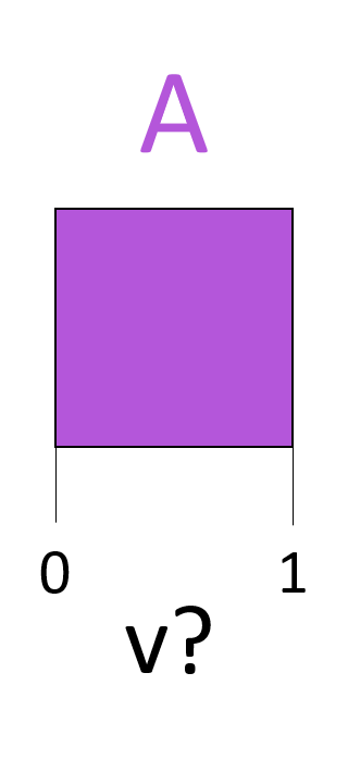
For $2^m$, let us first assume the value we are looking for is there. At each iteration it is possible that mid is either $v$, ending the algorithm, or not, halving the interval we are looking at. This continues until we either find $v$ at some iteration $i$ while there is still at least one value left, or we eventually arrive at our base case, where the last value is $v$.

If $v$ is not there, we will simply halve the interval $\log$ $n$ times and arrive at the base case anyway.
Now for our inductive step, which turns out to be pretty simple. Assuming $v$ is there, if it is not at the mid index, we half the interval, so we are now considering $2^{m+1-1}$ values, which is the same as $2^m$, which we have already shown is reducible to the base case.

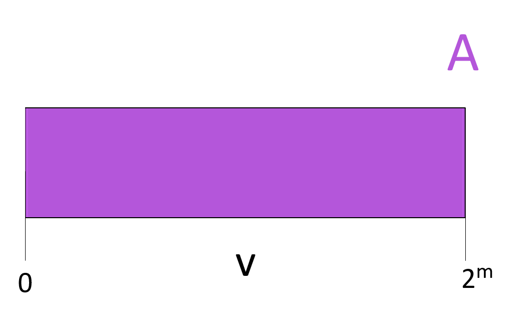
Otherwise, if $v$ is not present at all, we again move down to $2^m$ after one iteration, and then as previously shown, we will eventually end up at the base case and return $-1$.
Proof by Contradiction
Proof Idea
In order to prove an algorithm by contradiction, we must identify invariant properties of the algorithm that must be true in all cases. Then with these, we will try to imagine scenarios where they would be false, but then show that these scenarios actually contradict some property of the algorithm. The properties we will use are that if $v$ is in $A$, then every [left, right] range considered in the running of the algorithm must contain $v$, that if mid is $v$, then the algorithm returns the index, and that if mid is not $v$, the algorithm will choose the left side if $v$ is less than mid and the right side if $v$ is greater than mid.
Proof Details
First, let’s consider if $v$ is not in $A$ to begin with. This means for the algorithm to be false, a valid index should be returned despite $v$ not being present. With the way the algorithm runs, however, the only way to return an index instead of $-1$ is if mid = v is true. This only happens when the current mid value of the range is $v$, which contradicts our statement that $v$ is not present.
Now, let’s assume that the algorithm is incorrect. This means that for some iteration, there exists a range [left, right] that $v$ is not in. At the beginning of the algorithm, left and right are assigned to the first and last values of the array. This raises a contradiction $-$ if $v$ is not in this range as we assumed, that would mean $v$ is not in $A$. This contradicts our statement that $v$ is in $A$.
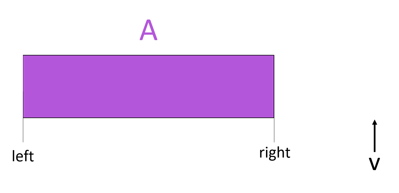
Let’s now look at the first iteration $i$ (smallest $i$) where $v$ is in $A$ but not in the current range. In order for our algorithm to be incorrect, $v$ must not be in this range. In order for this to happen, the algorithm must have made a mistake at some point, and moved left when $v$ was greater than mid, or moved right when $v$ was less than mid. This is not possible however. In the code of the algorithm, the if statements move the interval left when $v$ is less than mid, and right when $v$ is greater than mid. This means $v$ must always be in the [left, right] range at any iteration, contradicting our assumption.
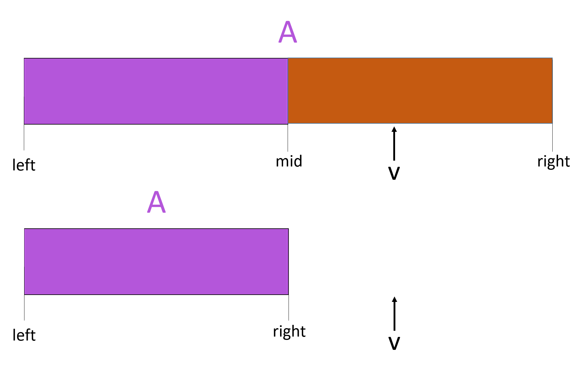
Lastly, if the algorithm is incorrect, it must fail to return the index when it finds $v$. This is easily contradicted by the algorithm, as if mid = v, it immediately returns the index. The other way it could be incorrect is if the algorithm returns $-1$ before it finds $v$. Since this only happens when left = mid = right, when the range has one value left, and since $v$ is always in the range, this would again need to say mid = v is false, which it cannot be.
Reduction
In the context of proofs, a reduction is essentially taking a problem and trying to prove that after some logical steps, it’s proof or answer is the same as a known problem. This is useful when you have a family of similar problems, because in some cases they have some shared property or limitation that is solved the same way across each one.
Imagine we have an array $A$ with $v$ where $v = a_0$. Binary search would actually be worse in this scenario, taking the full $O(\log n)$ time whereas a linear search will be $O(1)$. So this brings to light that as the array increases in size, if the index $v$ is at is significantly smaller than the size $n$ of the array, we are essentially searching a large portion of the array we don’t need to. How can we restrict binary search so it only searches as small a portion of the array as possible?
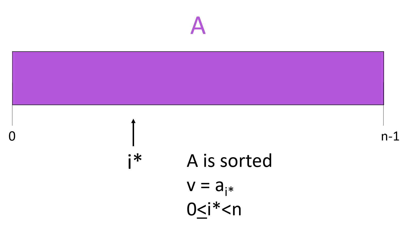
Let's define the problem like this:
Searching faster than Binary Search
- Array $A = [a_0, a_1, a_2, …, a_{n-1}]$ is sorted, and
- there exists $0 ≤ i^* < n$ such that $v = a_{i^*}$
The goal is to output $i^*$ in time $O(\log(i^*+1)+1)$.
Algorithm Idea
The general form of the problem is still in the realm of binary search $-$ we have a sorted array and we are looking for a specific value and outputing its index. This suggests there is some way we can get this problem into a form that regular binary search works on.
We can assume we know the left index for the search, since we can assume the array will start at index $0$. What we don’t know is what index to start right on. Let’s remember a property we found when proving binary search – if $v$ is in the array (we know it is), then the index of $v$ is contained in [left, right]. So we need to find a value $m$ such that $m$ is greater than $i^*$, then we can just do a binary search from $0$ to $m$. Knowing the value of $v$, we can look at the value of $a_m$ at each step to see if it is yet larger than $v$. Once $a_m$ is greater than $v$, we can stop. The way we can do this, and increase the running of the search by one iteration each time, is simply double $m$ at each step. This algorithm is then called Geometric Search.
Algorithm Details
Geometric Search
                                        //Input: A[0],...,A[n-1];v (A is sorted)

					m = 1

					while(A[m] < v)
					{
						m = min(m*2,n-1)
					}

                                        B = A[0:m]

					return binarySearch(B, v);
The important thing to notice here is that after determining $m$, we just run binary search kind of like calling a library function. This is the goal of a reduction $-$ taking an unsolved problem and reducing it to a form that is the same as a solved problem.
![If we increase m (yellow bar) until A[m] is greater than v, then we can use binary search](binarySearchImages/pic8.png)
Proof Idea
Kind of like importing a library into your code, we first can “import” our knowledge of binary search into our proof. From this we know the properties of binary search and the way it is solved. Now we need to prove that the steps we take to convert the problem into binary search are logically sound and that the resulting form is in fact binary search.
Using contradiction, we can show that by slowly increasing m, it eventually is the right bound for $i^*$ in binary search. We also need to show that the algorithm is efficient enough. The property we will explore here relates to how many times $m$ can be doubled, and how different variables dominate in Big-O notation.
Proof Details
First, we must show that after the first half of the algorithm, $i^* ≤ m$. To do this, let’s state that in order for the algorithm to be incorrect, the first loop must stop while $a_m$ is still less than $v$. This means that the condition of the loop, $a_m$ being less than $v$, is violated and the loop ends early. This is a contradiction. Therefore after that first loop, we can guarantee that $i^* ≤ m$ since $v = a_{i^*}$.
After this, we actually don’t need to prove anything new. Like how we used binary search as a black box in the algorithm, we can use the proof of correctness of binary search as a black box in the proof. Since we know that $v$ is in $A$, that $v=i^*$, and that $i^* ≤ m$, we can call upon the property of binary search where if $v$ is in a given range, then the search can find it. This is the final goal of the reduction $-$ we took a new problem and worked it down into a problem we already had algorithms and proofs for.
Runtime Analysis
The last thing we need to do is show that the algorithm is efficient enough. To do this, we show that the maximum value of $m$ is $2(i^*+1)$, which bounds how many iterations the algorithm will run for. If $i^*=0$, then the algorithm terminates at $m=1\le 2(i^*+1)=2$. Otherwise when $i^*>0$, we double $m$ each time we see that $a_m$ is less than $v$, meaning $m$’s maximum index must be some index whose value is less than $v$, then multiplied by $2$. We can thus simply say that this value must be less than $2i^*\le 2(i^*+1)$.
How many iterations of doubling is this? Well at iteration $j$, $m=2^j$, and if the final iteration is $j^*$, we know $2^{j^*}\leq2(i^*+1)$.
Now when taking $\log$ $2^{j^*}$, that reduces to just $j^*$, which then is at most $\log(2(i^*+1))=1+\log(i^*+1)$. Since each of the $j^*$ iterations take $O(1)$ time, the overall time before we call binarySearch is $O(j^*)\le O(1+\log(i^*+1))$.
Then the call to binarySearch is $O(\log(m+1))$, (since B is an array of size $m+1$), which is bounded from above by $ O(1+\log(i^*+1))$, so we simply state our overall runtime as $O((\log i^*+1) + 1)$, as desired.
Q3 on HW 0
Next, we will be reviewing the support page on matrix-vector multiplication with the goal of setting up some background for Q3 on HW 0. In particular, we will try and cover as much as the topic below as time permits:
- Definition of matrices and vectors.
- Example of a matrix-vector multiplication (time $O(n^2)$).
- Inner product
- Structured matrices
What is a Matrix?
In mathematics, a vector is simply an ordered list of values. A matrix represents a vector of vectors, or a 2-d vector. From the support page:
Matrices
A matrix $\mathbf{A}$ with $m$ rows and $n$ columns (also denoted as an $m\times n$ matrix) will in code be defined as int [][] A = new int[m][n] (assuming the matrix stores integers). Also a vector $\mathbf{x}$ of size $n$ in code will be declared as int [] x = new int[n] (again assuming the vector contains integers).
Note
For the Question 3 in HW 0, you are dealing with square matrices, i.e. $n=m$.
Matrix-Vector Multiplication
Given an $n\times n$ matrix $\mathbf{A}$ and a vector $\mathbf{x}$ of length $n$, their product is denoted by \[\mathbf{y} =\mathbf{A}\cdot \mathbf{x},\] where $\mathbf{y}$ is also a vector of length $n$ and its $i$th entry for $0\le i\lt n$ is defined as follows: \[y_i =\sum_{j=0}^{n-1} A[i][j]\cdot x[j].\]
The Inner Product
It turns out that to visualize the matrix-vector multiplication, it is helpful to define a simpler operation between two vectors:
Inner Product
Given two vectors $\mathbf{x}$ and $\mathbf{y}$, both of length $n$, their inner product is defined as1 \[\left\langle \mathbf{x},\mathbf{y}\right\rangle = \sum_{i=0}^{n-1} x[i]\cdot y[i].\]
Armed with the definition of the inner product, here is an equivalent definition of the matrix-vector multiplication problem:
Matrix-vector multiplication (redefined)
Given an $n\times n$ matrix $\mathbf{A}$ and a vector $\mathbf{x}$ of length $n$, their product $\mathbf{y}=\mathbf{A}\cdot\mathbf{x}$ can also be defined as follows. Its $i$th entry for $0\le i\lt n$ is defined as follows: \[y_i =\left\langle \mathbf{A}[i],\mathbf{x}\right\rangle,\] where $\mathbf{A}[i]$ denotes the $i$th row of $\mathbf{A}$.
Below is one example of a matrix vector multiplication: \[ \begin{pmatrix} 1 & 2 & -3\\ 2 & 9 &0\\ 6 & -1 & -2 \end{pmatrix} \times \begin{pmatrix} 2\\ 3\\ -1 \end{pmatrix} = \begin{pmatrix} 1\times 2 + 2\times 3 + (-3)\times(-1)\\ 2\times 2+ 9\times 3+0\times (-1)\\ 6\times 2+(-1)\times 3+ (-2)\times(-1) \end{pmatrix} = \begin{pmatrix} 11\\ 31\\ 11 \end{pmatrix}. \]
Time Complexity
The time complexity of a regular multiplication is $O(n\cdot m)$, or $O(n^2)$ for square matrices. You can think of it as being two nested for loops. One for each row, and the inner one for each column. Here is a pseudocode example of multiplying matrix $\mathbf{A}$ with vector $\mathbf{x}$:
Algorithm Details
                                    Allocate an array of length n and call it y

                                    #Initialize the array
                                    for i= 0 .. n-1
                                        y[i]=0

                                    #Do the actual matrix-vector multiplication
                                    for i = 0 .. n-1
                                        for j= 0 .. n-1
                                            y[i] += A[i][j] * x[j]

                                    return y
In-recitation Exercise
Run the above algorithm on the matrix-vector multiplication example from last section. Also argue this is an $O(n^2)$ algorithm.
Structured Matrices
If we know what the structure of a matrix is, we can often cut down on our algorithm time. We will consider one such example below and Question 3 on HW 0 is also based on this theme.
Outer Product
Outer Product
Given two vectors $\mathbf{s}$ and $\mathbf{t}$, their outer product is defined as the $n\times n$ matrix $\mathbf{A}$ such that for any entry $(i,j)$, we have \[A[i][j]=s[i]\cdot t[j].\]
In-recitation Exercise
Show the computation of the outer product of $\mathbf{s}=[4, 3, 2]$ and $\mathbf{t}=[-3, 2, 1]$.
Next, we present an algorithm to multiply the outer product of two arbitrary vectors $\mathbf{s}$ and $\mathbf{t}$ with a vector $\mathbf{x}$ in time $O(n)$. (Note that this is a significant improvement over the runtime from the trivial algorithm above.) In other words, we want to solve the following problem
Multiplying outer product with a vector
Given three vectors $\mathbf{s},\mathbf{t}$ and $\mathbf{x}$, compute the product of the outer product of $\mathbf{s}$ and $\mathbf{t}$ with the vector $\mathbf{x}$. If $\mathbf{y}$ is the product, then it is defined as (for every $0\le i\lt n$): \[y_i=\sum_{j=0}^{n-1} s[i]\cdot t[j]\cdot x[j].\]
Algorithm Idea
Observe that \[y_i=\sum_{j=0}^{n-1} s[i]\cdot t[j]\cdot x[j]=s[i]\cdot \sum_{j=0}^{n-1} t[j]\cdot x[j] = s[i]\left\langle \mathbf{t},\mathbf{x}\right\rangle.\] In other words, once we have computed $\left\langle \mathbf{t},\mathbf{x}\right\rangle$, one can compute $y_i$ by just multiplying the inner product with $s[i]$, which takes $O(1)$ time for each $0\le i\lt n$.
In-recitation Exercise
Do a run of the above algorithm on $\mathbf{s}=[4, 3, 2]$, $\mathbf{t}=[-3, 2, 1]$ and $\mathbf{x}=[3, 2, -2]$.
In-recitation Exercise
Compare the answer from the previous exercise to the answer you get when using our original algorithm with the outer product matrix.
In-recitation Exercise
The runtime for this algorithm is $O(n)$? Why?
Further Reading
- Make sure you carefully read the policy documents: Syllabus and Homework policies.
- Support page on proofs.
- Proof by induction support page.