HW 6, Question 1

Part (a)

This part is fairly straightforward so we'll keep it short and sweet:

                                            #Inputs: non-negative integers a and n

                                                ans = 1
                                                for i = 1 to n
                                                    ans *= a

                                                return ans
                                        

Part (b)

We start with an important reminder:

Recurrence Relations

$T(n) = T(n/2)+O(1)$

We start off with the Binary search algorithm (stated as a divide and conquer algorithm):

                                        // The inputs are in A[0], ..., A[n-1]; v

                                        l = 0
                                        r = n-1
                                        return binary_search(A,l,r,v)
        
                                        # Recursive definition of Binary Search
                                        def binary_search(A,l,r,v):

                                            if l == r:
                                                return v == A[l] # Return 1 if A[l]=v and 0 otherwise
                                            else:
                                                m = (l-r)/2
                                                if v <= A[m]:
                                                    return binary_search(A,l,m,v)
                                                else:
                                                    return binary_search(A,m,r,v)
                                        

It is easy to check that every line except the recursive calls of binary_search takes $O(1)$ time. So if $T(n)$ is the runtime of binary_search, then it satisfies the following recurrence relation:

Next, we will argue the following

Proof Idea

The idea is to unroll the recurrence. Each level has a contribution of $c$:

.

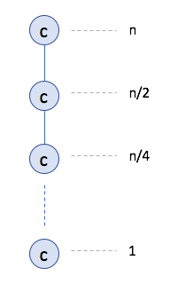
Since there are at most $\log_2{n}+1$ levels, this implies the claimed bound.

$T(n) = T(n/2) +O(n)$

We now consider the following recurrence relation

The book on Page 219 solves this recurrence. We do a very quick overview now.

We do the "unroll the recurrence and use the pattern technique." At an arbitrary level $j$, there is one instance, of size $\frac{n}{2^j}$ and contributes $\frac{cn}{2^j}$ to the recurrence relation. Thus, we have (for $n\ge 2$): \[T(n)\le \sum_{j=0}^{\log_2{n}} \frac{cn}{2^j} =cn\cdot \sum_{j=0}^{\log_2{n}} \frac{1}{2^j}.\]

Working out this geometric sum, we will find that it converges to $2$. Thus, we can say, for recurrence relation 2 above we have \[T(n) \le 2cn \le O(n).\]

HW 6, Question 2

Part (a)

Even though it is not needed for this problem, we next present a more detailed proof:

Part (b)

Integer Multiplication (Re-explained)

The setup

We first recall the problem that we are trying to solve:

Next, recall the following notation that we used: \[a^0 = \left(a_{\lceil\frac{n}{2}\rceil-1},\dots, a_0\right),\] \[a^1 = \left(a_{n-1},\dots, a_{\lceil\frac{n}{2}\rceil}\right),\] \[b^0 = \left(b_{\lceil\frac{n}{2}\rceil-1},\dots, b_0\right),\] and \[b^1 = \left(b_{n-1},\dots, b_{\lceil\frac{n}{2}\rceil}\right).\] Next, we try and reason about the $O\left(n^{\log_2{3}}\right)$ algorithm using polynomials (in one variable) .

Enter the Polynomials

We begin by defining two polynomials \[A(X) = a^1\cdot X + a^0,\] and \[B(X) = b^1\cdot X + b^0.\] To situate these polynomials, we make the following observations (make sure you are comfortable with these):

Now let \[C(X)= A(X)\cdot B(X),\] be the product of the two polynomials. Then note that by Exercise 1, we have that our final answer can be read off as \[c = C\left(2^{\lceil\frac{n}{2}\rceil}\right).\] Next, note that $C(X)$ is a polynomial of degree two and hence can also be represented as \[C(X) = c^2\cdot X^2+c^1\cdot X+c^0.\] Recall the fact that $C(X)=A(X)\cdot B(X)$ we also have \[C(X) = \left(a^1\cdot X+a^0\right)\cdot \left(b^1\cdot X+b^0\right) = \left(a^1\cdot b^1\right)\cdot X^2 + \left(a^1\cdot b^0+a^0\cdot b^1\right)\cdot X+\left(a^0\cdot b^0\right).\] By comparing the coefficient of the powers of $X$, we get that \[c^2 = a^1\cdot b^1,\] \[c^1 = a^1\cdot b^0+a^0\cdot b^1\] and \[c^0 = a^0\cdot b^0.\]

Now going back to the algorithm

The important observation is that in our divide and conquer algorithm the three recursive calls are so that we can compute $c^0, c^1$ and $c^2$. For $c^0$ and $c^2$, the recursive calls are obvious. It is for the case of computing $c^1$ that we needed the supposed "clever" identity

Now of course one can verify that the identity is correct and it works for our case. But here is another way to arrive at the identity (that uses all the polynomial stuff that we have been talking about so far). In particular consider $C(1)$. Note that we have \[C(1) = c^2+c^1+c^0.\] In other words, we have \[c^1 = C(1) - c^2 - c^0.\] Finally, note that $C(1) = A(1)\cdot B(1) = (a^1+a^0)(b^1+b^0)$ and using this in the above (along with the values of $c^2$ and $c^0$) proves the identity.

Um, why is this any better?

Finally, we give some argument to justify why the argument using polynomials is more "natural." Note that

1. We needed to compute the coefficients of the polynomials $C(X)$.
2. For any constant value $\alpha$ (e.g. $\alpha=1$) both $A(\alpha)$ and $B(\alpha)$ are numbers with roughly $n/2$ bits and hence $C(\alpha)$ can be computed with multiplication of two numbers with roughly $n/2$ bits.

To complete the last piece of the puzzle, we invoke polynomial interpolation . In particular, to compute the coefficients of $C(X)$ we only need the evaluation of $C(x)$ at three distinct points (each of which corresponds to multiplication of two roughly $n/2$-bit numbers). Indeed this is what has been happening above:

1. First note that $C(0) = A(0)\cdot B(0)=c_0$.
2. Recall we used $C(1) = A(1)\cdot B(1) = c^2+c^1+c^0$.
3. Finally, we can interpret $c^2$ as $\lim_{X\to\infty} \frac{C(X)}{X^2}=\lim_{X\to\infty} \frac{A(X)}{X}\cdot \lim_{X\to\infty}\frac{B(X)}{X}$ and in a hand wavy way we can think of recovering $c^2$ by "evaluating" $C(X)$ at infinity.

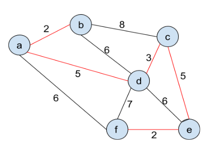
Prim's Algorithm

Similar in functionality to Dijkstra's algorithm.

Example

Run Prim's algorithm on the input:

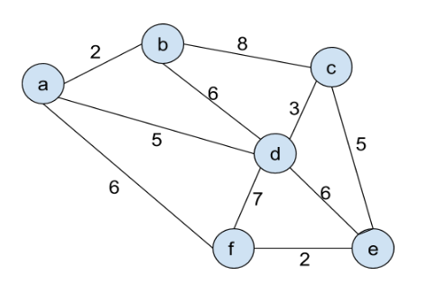
The following is the output:

Further Reading

• Section 5.2 in the textbook.
• Support page on integer multiplication.