Recitation 7
Recitation notes for the week of March 5, 2025.
Minimizing Maximum Lateness
This problem is relevant to HW 4, Q3!
We will not cover the minimizing maximum lateness problem in any detail in class. Please read up the care package on this problem.
Problem Statement
Here is a quick recap of the problem statement:
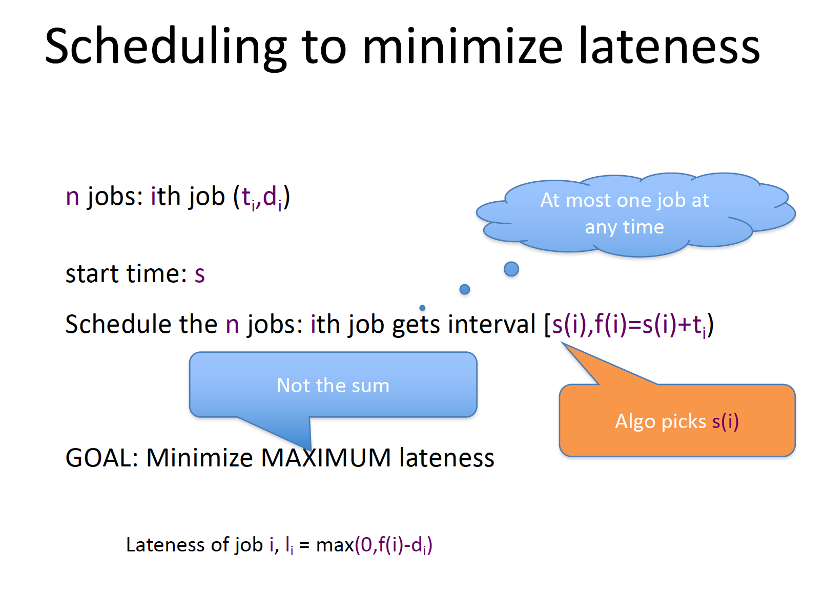
Input Instance
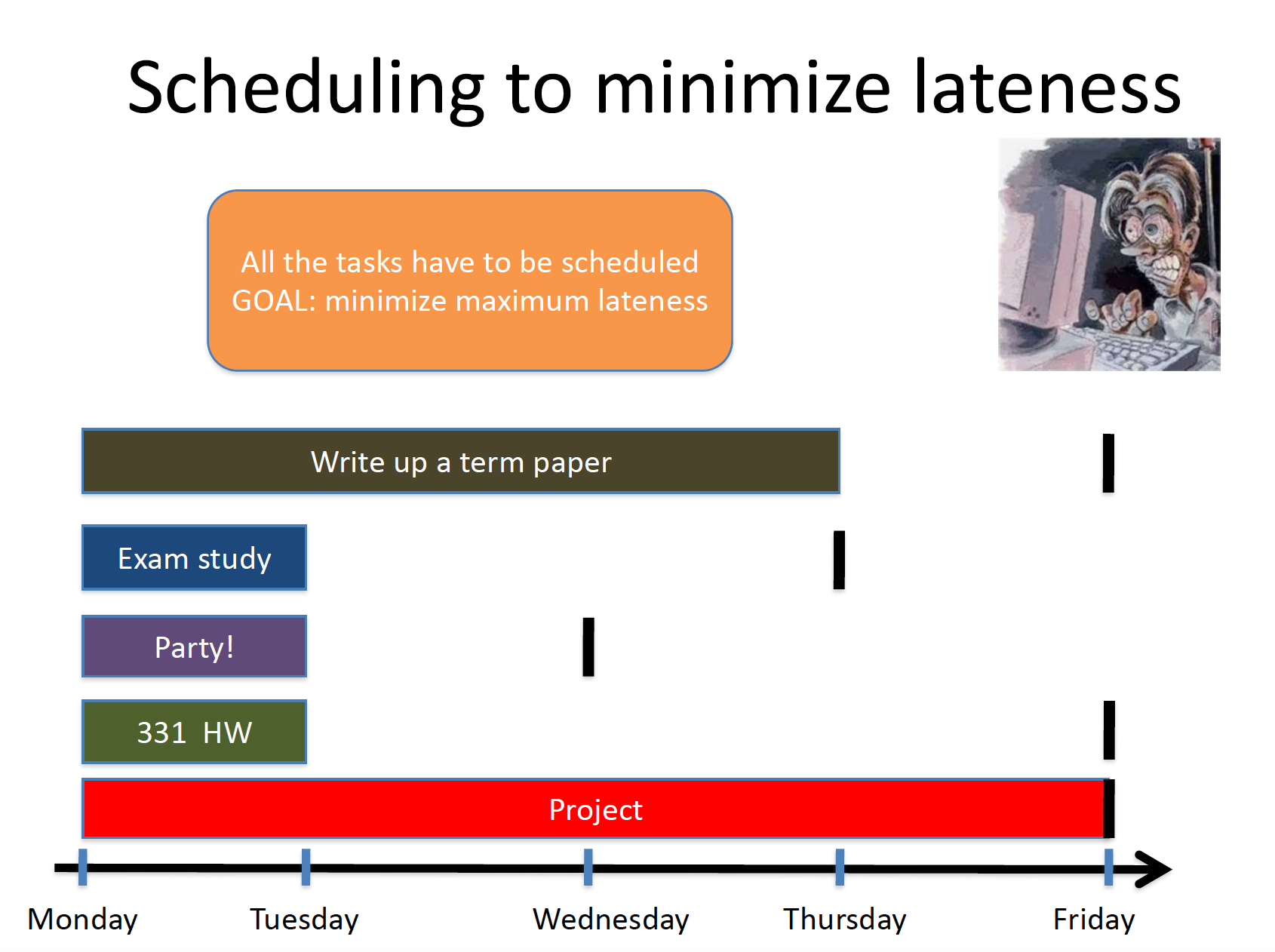
Here is an example input to the problem:
Input Instance
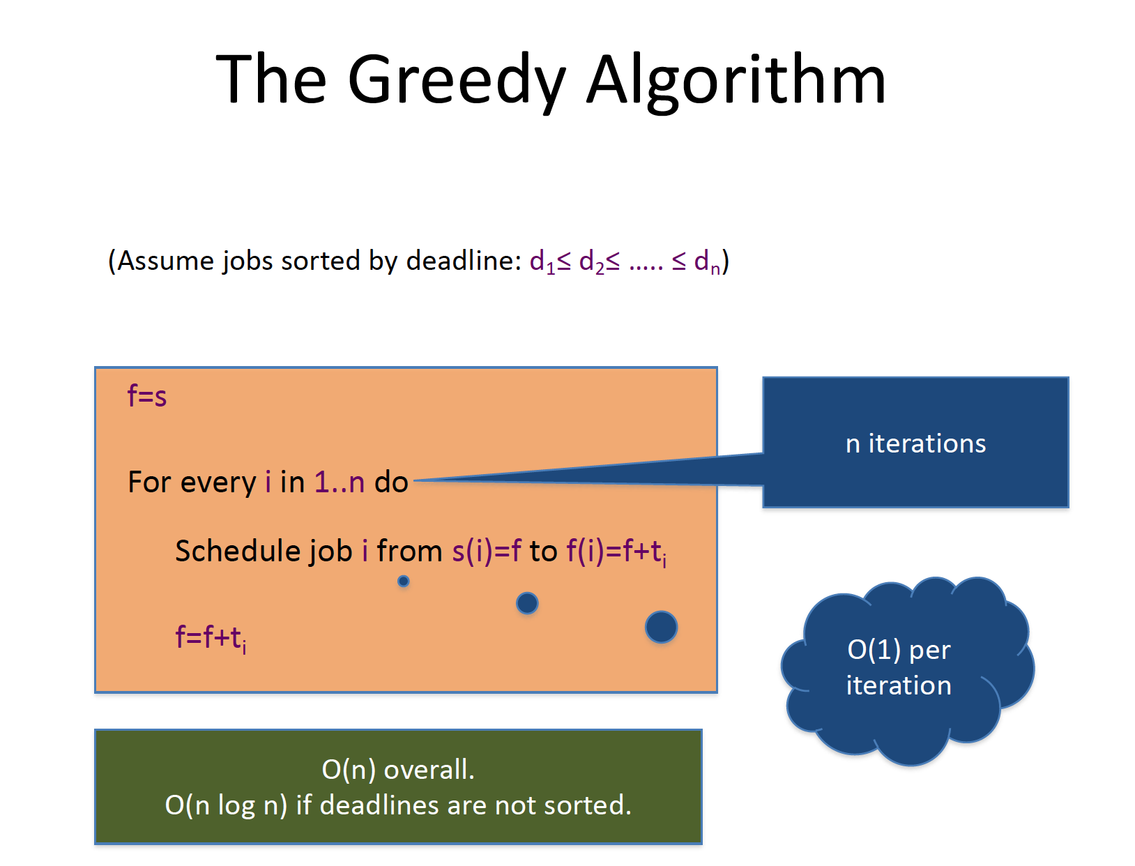
Here is the greedy algorithm to solve the problem:
Exercise
Run the greedy algorithm on the above instance and calculate lateness of each job (assuming one breaks ties for jobs with "Friday" as deadline in order 331 HW, Write up a term paper and Project) and compute the final maximum lateness (which should be $6$ for Project job).
HW 4, Question 1
We begin by restating the problem statement:
The Problem
We come back to the issue of Wall Maria needing alarms for warning soldiers of an imminent titan attack. In this question, you will consider an algorithmic problem that you would need to solve to help out Survey Corps install alarms.
After lots of rounds of discussions and public feedback, it was decided that the most cost-effective way to install alarms on Wall Maria was to put them into the beam towers of the wall. There are two things in your favor:
- The Wall Maria can be considered a straight line.
- The above implies that you only need alarms that need to broadcast their signal in a narrow, linear range, which means an alarm can be heard by all the beam towers within $70$ miles ahead from its location. These alarms are unidirectional so they can provide sound to only beam towers that are ahead of it.
You will design an efficient algorithm, which your team can use to figure out which beam towers should have alarms installed in them so as to use the minimum number of alarms.
With an eye on the future, the alarms have to be placed so that there is continuous sound coverage on the wall from the first and the last beam tower of the wall. I.e. it should never be the case that you are on the wall (between the first and the last beam tower) such that you are
strictly more than $70$ miles ahead of the closest alarm. You can assume that you have to put an alarm at a first starting beam tower, which will be reference point to all other subsequent beams, on Wall Maria.
Note
You should assume the following for your algorithm:
- No two consecutive beam towers are more than $69$ miles apart. Note that this implies there always exists a feasible way to assign alarms to beam towers. Further, note that beam towers can be much closer than $69$ miles to each other.
- The input to your algorithm is a list of beam towers along with their distance (in miles) from the very first beam. You cannot assume that this list is sorted in any way.
Here are the two two parts of the problem:
- Part (a): Assume that we relax the condition that the alarms have to be next to a beam tower: i.e. you can place an alarm anywhere in between beam towers (the $70$ mile coverage restriction on the alarms still applies). Design an $O(n)$ time algorithm to solve this related problem.
- Part (b): Design an $O(n\log{n})$ time algorithm to solve the original problem (i.e. where the alarms have to in a beam tower). Prove the correctness of your algorithm and analyze its running time.
We begin with an example input to show the solutions to both part (a) and (b) (and in particular, pointing out why solving part (a) does not solve part (b)):
Sample Input/Outputs
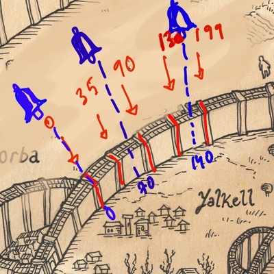
- Input:
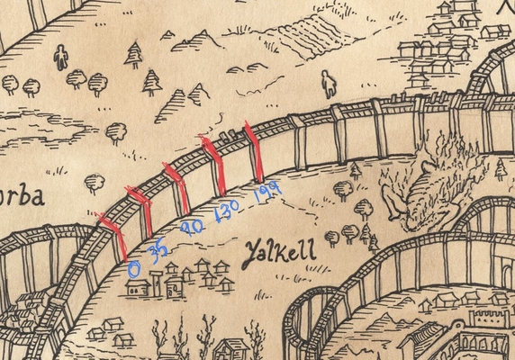
In the above $n=5$ and we have an alarm at the first beam tower since that is mandated by the problem. Also note that any two consecutive beam towers are at most $69$ miles apart . Note that in this case a valid input your algorithm should handle is $[ (1, 35), (2, 90), (3, 130), (4, 199) ]$, where in each pair the first index refers to a beam tower (so in the example above the beam towers in order are $1,2,3,4$) and the second element of a pair is the distance in miles from the first beam tower.
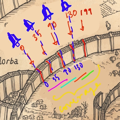
- Solution for part (a): Here is an optimal solution for part (a) for the above input:
Here is a quick visual argument for the above leads to continuous sound coverage:

We will see shortly that this is an optimal assignment for part (a).
- Solution for part (b): Here is an optimal solution for part (b) for the above input:
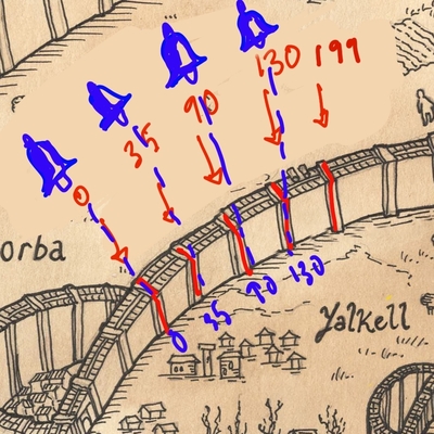
Here is a quick visual argument for the above leads to continuous sound coverage:
We will not prove it, but this is an optimal assignment for part (b).
Part (a)
Algorithm Idea
The idea is very simple: since we do not have any restriction on where the alarms can be placed: we will place them at multiple of $70$ mile marks till there is continuous coverage from the first to the last beam tower.
Even though it is not needed for the HW submission
We provide the algorithm details and proof of correctness idea below for your convenience.
Algorithm Details
                                    //Input is (h1,d1), ... , (hn-1,dn-1)
                                    // di is the distance of beam tower hi from the first beam tower

                                    dmax= max(d1, ... ,dn-1)

                                    d=0 //Assuming the first beam tower is at mile 0
                                    while( d < dmax)
                                        Place an alarm at mile d
                                        d += 70
Proof (of Correctness) Idea
First note that the algorithm above places $\left\lceil \frac{d_{\max}}{70}\right\rceil$ many alarms.
To complete the proof, we claim that any valid placement of alarms must place at least $\left\lceil \frac{d_{\max}}{70}\right\rceil$ alarms. For the sake of contradiction assume that we are able to come up with a valid placement with \[\le \left\lceil \frac{d_{\max}}{70}\right\rceil -1 < \frac{d_{\max}}{70}\] alarms. Since each alarm can cover $70$ miles, this means that the total number of miles covered will be \[<70\cdot \left(\frac{d_{\max}}{70}\right) = d_{\max},\] which means at least $1$ mile from the first beam tower and the last beam tower does not have sound coverage, which means that our placement was not valid.
Runtime analysis
We will assume the following, which you need to prove on your own:
Exercise 1
\[d_{\max}\le 69n.\]
while runs for at most $69n/70\le n$ times. Each iteration takes $O(1)$ time: so overall the loop takes $O(n)$ time. Since computing $d_{\max}$ takes $O(n)$ time, the overall runtime is $O(n)$, as desired.
Part (b)
We would like to point out two things:
- The algorithm above for part (a) does not work for part (b). The basic idea is that the algorithm from part
(a) can place an alarm at a mile where there is no beam tower but for part (b) the alarms have to be at a beam tower. See the sample input/output above for a concrete example. - Think how you could modify the algorithm for part (a) could be modified to handle the extra restriction that the alarms have to placed next to a beam tower.
Hint
Think of a greedy way to decide on which beam towers to pick for alarm installation. It might help to forget about the scheduling algorithms we have seen in class and just think of a greedy algorithm from "scratch." Then try to analyze the algorithm using similar arguments to one we have seen in class.
Note
The proof idea for part (a) does not work for part (b): you are encouraged to use one of the proof techniques we have seen in class to prove correctness of a greedy algorithm.
Greedy Stays Ahead
We briefly (re)state the greedy stays ahead technique in a generic way (and illustrate it with the proof of the greedy algorithm for the interval scheduling problem that we saw in class).
Roughly speaking the greedy stays ahead technique has the following steps:
Sync up partial greedy and optimal solutionGreedy algorithms almost always build up the final solution iteratively. In other words, at the end of iteration $\ell$, the algorithm has computed a `partial' solution $\texttt{Greedy}(\ell)$. The trick is to somehow `order' the optimal solution so that one can have a corresponding `partial' optimal solution $\texttt{Opt}(\ell)$ as well.Define a 'progress' measureFor each iteration $\ell$ (as defined above), we pick a 'progress' measure $P(\cdot)$ so that $P\left(\texttt{Greedy}(\ell)\right)$ and $P\left(\texttt{Opt}(\ell)\right)$ are well-defined. This is the step that is probably most vague but that is by necessity-- the definition of the progress measure has to be specific to the problem so it is hard to specify generically.Argue 'Greedy Stays Ahead' (as per the progress measure)Now prove that for every iteration $\ell$, we have \[P\left(\texttt{Greedy}(\ell)\right) \ge P\left(\texttt{Opt}(\ell)\right).\]Connect 'Greedy Stays Ahead' to showing the greedy algorithm is optimal. Finally, prove that with the specific interpretation of 'Greedy Stays Ahead' as above, at the end of the run of the greedy algorithm the final output is 'just as good' as the optimal solution. Note that the progress measure $P(\cdot)$ need not be the objective function that the greedy algorithm is trying to minimize (indeed this will not be true in most cases) so you will still have to argue another step to show that greedy stays ahead indeed implies that the greedy solution is no worse than the optimal one.
Next, we illustrate the above framework with the proof we saw in class that showed that the greedy algorithm for the interval scheduling problem was optimal:
Sync up partial greedy and optimal solutionWe did this by ordering the intervals in both the greedy and optimal solution in non-decreasing order of their finish time. Specifically, recall that we defined the greedy solution as \[S^*=\left\{i_1,\dots,i_k\right\}\] and an optimal solution as \[\mathcal O=\left\{j_1,\dots,j_m\right\},\] where $f(i_1)\le \cdots \le f_(i_k)$ and $f(j_1)\le \cdots f(j_m)$. With this understanding, the 'partial' solutions are defined as follows for every $1\le \ell\le k$: \[\texttt{Greedy}(\ell)=\left\{i_1,\dots,i_\ell\right\}\] and \[\texttt{Opt}(\ell)=\left\{j_1,\dots,j_\ell\right\}.\]Define a 'progress' measure. We define the progress measure as the (negation of) finish time of the last element in the partial solution, i.e. \[P\left(\texttt{Greedy}(\ell)\right) = -f\left(i_\ell\right)\] and \[P\left(\texttt{Opt}(\ell)\right) = - f\left(j_\ell\right).\] Two comments:- If the "$-$" sign in the definition of $P(\cdot)$ is throwing you off-- it's for a syntactic reason (and it'll become clear in the next step why this makes sense).
- Note that the progress measure above has nothing (directly) to do with the objective function of the problem (which is to maximize the number of intervals picked).
Argue 'Greedy Stays Ahead' (as per the progress measure). In class, we proved a lemma that stays that for every $1\le \ell\le k$, we have \[f\left(i_\ell\right)\le f\left(j_\ell\right).\] Note that this implies that for our progress measure (and this is why we had the negative sign when defining the progress measure), for every $1\le \ell\le k$, \[P\left(\texttt{Greedy}(\ell)\right) \ge P\left(\texttt{Opt}(\ell)\right),\] as desired.Connect 'Greedy Stays Ahead' to showing the greedy algorithm is optimal. For this step, we have a separate proof that assumed that if the 'Greedy Stays Ahead' lemma is true then $\left|S^*\right|\ge \left|\mathcal{O}\right|$.
A warning
Please note that while the above 4-step framework for the 'Greedy Stays Ahead' techniques works in many cases, there is no guarantee that this framework will always work, i.e. your mileage might vary.
HW 4, Question 2
This is Exercise $6$ in Chapter $4$: below is a quick summary (see the textbook for the details):
Ex. 6 in Chap. 4
There are $n$ campers, where each camper $i$ has a triple $(s_i,b_i,r_i)$. $s_i,b_i$ and $r_i$ are the times needed by camper $i$ for their swimming, biking and running legs of their triathlon. They have to do the three legs in order: swim first, then bike and then run. Only one camper can swim in the pool at a time but there is no such restriction on biking and running (i.e. if possible all campers can run/bike in "parallel"). Your goal is to schedule the campers: i.e. the order in which the campers start their swim leg so that the completion time of the last camper is minimized. I.e. you should come up with a schedule such that all campers finish their triathlon as soon as possible.
Sample Input/Outputs
- Input:
Say the input is $[(2,2,3),(2,3,4)]$, i.e. we have $s_1=2,b_1=2,r_1=3$ and $s_2=2,b_2=3,r_2=4$.
- Output:
Let us work this one out. There are only two schedules $1,2$ and $2,1$. So we consider both in turn:
- So assume camper $1$ starts at time $0$. They will get out of the pool at time $0+s_1=2$, will finish biking at the end of time $2+b_1=4$ and will finish the triathlon at the end of time $4+r_2=7$. On the other hand, camper $2$ starts at time $2$ (this is when camper $1$ is out of the pool). Camper $2$ will get out of the pool at time $2+s_2=4$, will finish biking at time $4+b_2=7$ and will finish triathlon at time $7+r_3=11$. Thus, the completion time of this schedule is $\max(7,11)=11$.
- Let us now consider the second schedule. In this case camper $2$ starts first and finishes at time $0+2+3+4=9$ and camper $1$ starts at time $2$ and finishes at $2+2+2+3=9$. Thus, the completion time in this case is $\max(9,9)=9$.
Part (a)
Here we have to argue that there is always an optimal solution with no idle time: i.e. there should be no gap between when a camper finishes their swim and when the next camper starts their swim.
Proof Idea
Assume that camper $i$ has start time $st_i$. Note we want to argue that for every $i$, $st_{i+1}=st_i+s_i$. If this condition is satisfied for all $i$, them we are done. So assume not. We will now show how to convert this into another set of start times $st'_i$ for every camper $i$ that has no idle time and the resulting schedule is still optimal. Repeat the following till there exists a camper $i$ such that $st_{i+1}> st_i+s_i$-- update $st_{i+1}=st_i+s_i$. Once this procedure stops, let $st'_i$ be the final start time of camper $i$.
Let $c_i=st_i+s_i+b_i+r_i$ be the original finish time for camper $i$ and let $c'_i=st'_i+s_i+b_i+r_i$ be the new finish time. Then one can argue by induction that (and this is your exercise):
Exercise 2
For every camper $i$, $c'_i\le c_i$.
Part (b)
Note
Part (a) actually then shows that we only need to figure out the order of the campers: once that is set, the start times are automatically fixed. Hence for part (b), one just needs to output the ordering among the campers.
In this part you have to come up with an efficient (i.e. polynomial time) algorithm to come up with an optimal schedule for the campers that minimizes the completion time. We repeat the following note and hint from the problem statement:
Note
As has been mentioned earlier, in many real life problems, not all parameters are equally important. Also sometimes it might make sense to "combine" two parameters into one. Keep these in mind when tackling this problem.
Hint
In the solution that we have in mind, the analysis of the algorithm's correctness follows the exchange argument. Of course that does not mean it cannot be proven in another way.
Exchange Argument for Minimizing Max Lateness
Main Idea
If we have a schedule with no idle time and with an inversion, then we can rid of an inversion in such a way that will not increase the max lateness of the schedule.
Recall
In (4.8) in the book, we showed that schedules with no inversions and no idle time have the same max lateness.
Given the schedule below where the deadline of $j$ comes before the deadline of $i$ (the top schedule has an inversion):
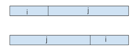
Let us consider what happens when we go from top schedule to the bottom schedule. Obviously $j$ will finish earlier so it will not increase the max lateness, but what about $i$? Now $i$ is super late.
However, note that $i$’s lateness is $f(j) - d(i)$ where $f(j)$ is the finish time of $j$ in the top schedule. Now note that \[f(j) - d(i) < f(j) - d(j),\] so the swap does not increase maximum lateness.
An Example
Here is an explicit example showing the above proof argument: \[d(a) = 2~~~~ t(a) = 1\] \[d(b) = 5~~~~ t(b) = 6\] \[d(c) = 8~~~~ t(c) = 3\]
Now consider this schedule with inversions: \[__a__|____c____|______b_______\] And another schedule without inversions: \[__a__|______b_______|____c____\]
The first schedule has max lateness of $5$ while the second schedule has max lateness of $2$.
NOTE
Examples do not suffice as proofs. But they are good for understanding purposes.