CSE4/587 Spring 2017
Data-intensive Computing = Data Science + Big Data Infrastructure
| Date | Topic | Chapter | Classnotes | To do: |
|---|---|---|---|---|
| 1/30 | Course Goals and Plans | Course description | C1 | Read Ch.1 |
| 2/1 | Data science process, data and data collection methods | Chapter 1,2 | C2 | Install Jupyter |
| 2/6 | Working with R Kernel on Jupyter. Lab1 Discussion | Chapter 1,2 | R on Jupyter | Work on Lab1 |
| 2/6 | Exploratory Data Analysis (EDA) | Chapter 2 | nyt2.csv | Work on NYTimes Click Rate Data Ch.2 |
| 2/13 | Data Cleaning | Chapter 2; Intro to R Studio | manhat.csv (Titanic) train.csv(Titanic) test.csv | Manhattan Data; Titantic Data |
| 2/15 | Algorithms for Data Processing | Chapter 3; Demos with R Studio | cars datasetand a generated dataset | Analysis, Visualization and interpretation using Linear Regression |
| 2/20 | Algorithms for Data Processing: K-NN | Chapter 3; Lab 2 discussion | Lab 2: Data Cleaning | Analysis using K-NN |
| 2/24 | Algorithms for Data Processing: K-means | Chapter 3; Revisit K-NN; Lab 2 discussion | Lab 2: Data; What to do? (Take 2) | Analysis using K-Means | 2/27 | Lab 2 questions | Lab 2 discussion | Lab 2: Data; What to do? (Take 3) | Activity 3 and 4 |
Exploratory data analysis
Lets review what we did last class: we discussed Lab1.
1. Please make sure your work environment is ready. See the installation handout
2. We have a verified answer for the issue of location of tweets. See project handout. and also twitteR manual.
Today we will look into exploratory data analysis with actual data from Nytimes click rate.
What is EDA? Developed by John Tukey of Bell Labs. EDA is a first step in building a model. This involves plots, graphs and summarization to develop a general understanding of the problem.The data provided with your text has data from NYTimes homepage clicks for 31 days (May 2012). It is about 100000 observations of 5 varaibles each for each day. Lets perform an EDA to understand the problem and the data. You can download the data from here.
I will type in, run and annotate every step. See pages 39-40 of your text.
Data Cleaning (and Transformation)
Today's plan:
- Lets review Lab1 ques and answers
- Intorduction to RStudio and some of its features
- Data cleaning of real estate sales data
- Data transformation in titanic data
- Data for today's demo
Please see recitaion and office hours schedule posted on Piazza
We are still in Chapter 2. Today we will look at Data Cleaning and EDA for another real business: http://www.realdirect.com It is "Rethinking real estate": how it is bought/sold. This is a real estate business based on a subscription model. Traditional model involves a broker and a hefty commision for the broker selling the house (anywhere between 7-10%). RealDirect will provide.
- Broker support and interface and data-analytics intelligence
- Seller interface: sellers "subscribe" to realdirect (flat fee $365 month)
- Sellers get brokers at a lower rate (1%-2%)
- Buyers can use realdirect interface/platform to search, negotiate, and buy the available listing. (active, offer made, in contract, offer rejected etc.)
Cleaning Data: Basic steps
- Convert unknown file types to csv. For example, excel does read well into R, so convert it to csv and read it in as csv file.
- Remove characters such as $ and , embedded within numeric data
- Turn all (or select) variable names as well as values to lowercase for easy comparison and processing
- Remove outliers, zeros and N/A (blanks)
- Transform characters to numeric code
- Binning or categorizing data: add variable(s) that will "bin" or "categorize" orginal data. Example: age$Cat (-Inf,0, 10,30,50,inf)
- Add new information columns: "class" or "levels"
- Remove unwanted observations, and variables
- Add meaningful labels to support charting (this is more an EDA step)
- Turn character/quantitative data into factors
Algorithms for Data Processing I
Today's plan:
- Lets review Lab1 questions and answers: dropping widgets? There is a solution, RShiny, too late for lab1. We will do it later labs.
- Algorithms for data processing: we will learn just one of these today
- Linear regression (linear model): a versatile algorithmic approach
- Famous "R cars data package": "lm" demo
- Synthesizing data using R methods: contrarian "lm" demo
Please see recitaion and office hours schedule posted on Piazza
Motivation 1 for "lm": Here is a list of Top ten machine learning algorithms.
Motivation 2 for "lm": Bloomberg's oil price prediction method.
We are in Chapter 3. Read Chapter 3. Three important data processing algorithms are discussed in this chapter. We will look into just one of these today: Linear Regression. Problem 1: Consider the data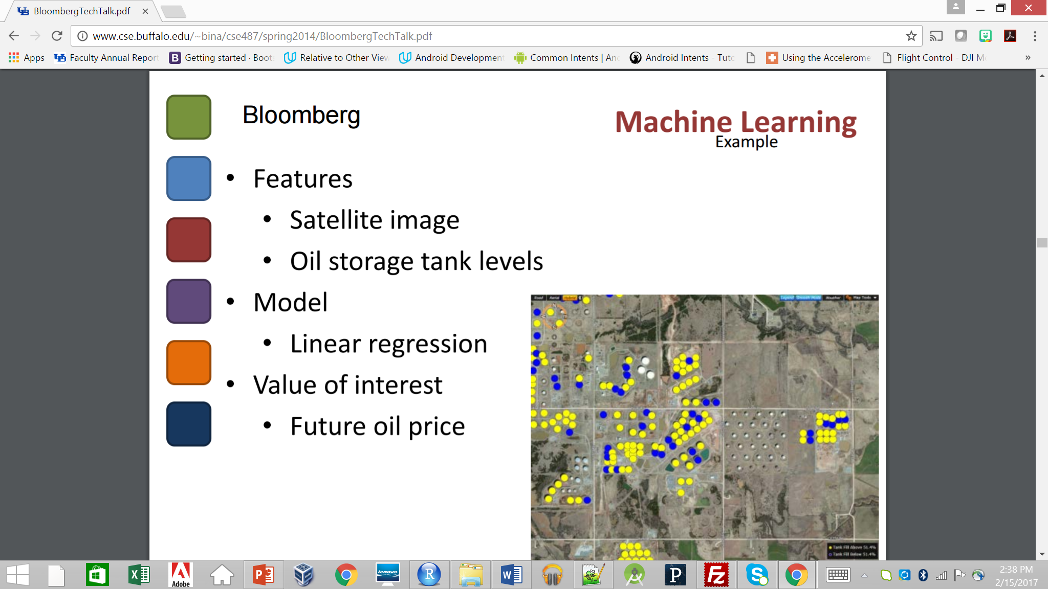
S = {(x,y)= (1,25), (10,250), (100,2500), (200,5000)}What next? What is value for X = 40? We observe that
- There is a linear pattern.
- Coefficient relating x and y is 25
- Seems deterministic
- and y = 25*x is the relationship, an obvious linear pattern.
Linear model is defined by the functional form:
y = β0 + β1*x
- A simple analysis of "cars" data already available in R environment Another demo to understand the evaluation metric for an "lm" . Goal is to visualize and understand lm and its statistics.
- The second demo is on synthetic data to understand the importance of the evalaution metrics and also to understand "overfitting"
- Cleaning and getting a data frame
- Plot the data points
- Visually assess the data plot
- Model using "lm"
- "lm" by default seeks to find a trend line that minimizes the sum of squares of the vertical distances between the approximated or predicted and observed y's.
- We want to learn both the "trend" and the "variance"
- Evaluate the measure of goodness of our model in R-squared and p: R-square measures the the proportion of variance. p-value assesses the significance of the result. We discuss both these measures: we want R-sqaured to high (0.0-1.0 range) and p to be low or <0.05. R-squared is 1-(total predicted error-squared/total mean error squared) (see p.67)
See Demo code here
Algorithms for Data Processing II
Today's plan:
- Introduction to Lab2 and discussion.
- Evaluation metric for linear regrssion
- K-NN: K-nearest neighbor
- Demo K-nn, mis-classification rate and prediction
Linear Regression Evaluation Metric
1. Goodness of fit:
R2 range is 0-1. For a good fit we would like R2 to be as close to 1 as possible. R2 = 1 means every point is on the linear regression line!
The second term represents the "unexplained variance" in the fit. You want this to be as low as possible.
2. Quality of data p: Low p means Null hypothesis (H0) has been rejected. We would like p <0.05 for high significance of prediction.
K-NN Algorithm
- K-nearest neighbor
- Supervised machine learning
- You know the “right answers” or at least data that is “labeled”: training set
- Set of objects have been classified or labeled (training set)
- Another set of objects are yet to be labeled or classified (test set)
- Your goal is to automate the processes of labeling the test set.
- Intuition behind K-NN is to consider K-closest items for similarity --- similarity defined by their attributes, look at the existing label and assign the test object the label.
Intuition
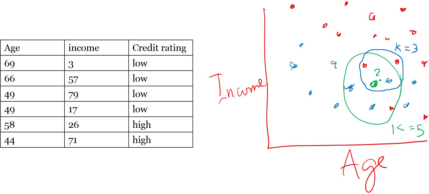
K-NN Issues
- How many nearest neighbors? In other words what is the value of k
Small K: you overfit
Large K : you may underfit
Or base it on some evaluation measure for k choose one that results in least % error for the training data (we will do this in today's demo) - Implications of small k and large k
- How do define similarity or closeness?
Euclidian distance
Manhattan distance
Cosine similarity etc. - Error rate or misclassification (k can be chosen to lower this)
- Curse of dimensionality
See Demo code here
Algorithms for Data Processing III
Today's plan:
- Lab2 discussion: Where is the data?
- Hmm.. the question of normalization of data in K-NN
- Look at small data set by hand and on R Studio
- K-Means Clustering
- Demo K-Means; Evaluation metric.
Lets Review K-NN
General idea is that a data point will similar to its neighbors. So classify it or label it accordingly. Which neighbor(s), how many neighbors? Here is an overview of the process:- Decide on your similarity or dsitance metric
- Split the original set into training and test set
- Pick an evalaution metric: Misclassification rate is a good one
- Run K-NN few times, changing K and checking the evaluation metric
- Once best K is chosen, create the test cases and predict the labels for these
Manhattan distance (X+Y) is another, data need not be normalized. Hamming, Cosine distance are other. See many others discussed in text p.76.
Lets try it out with a sample data set:
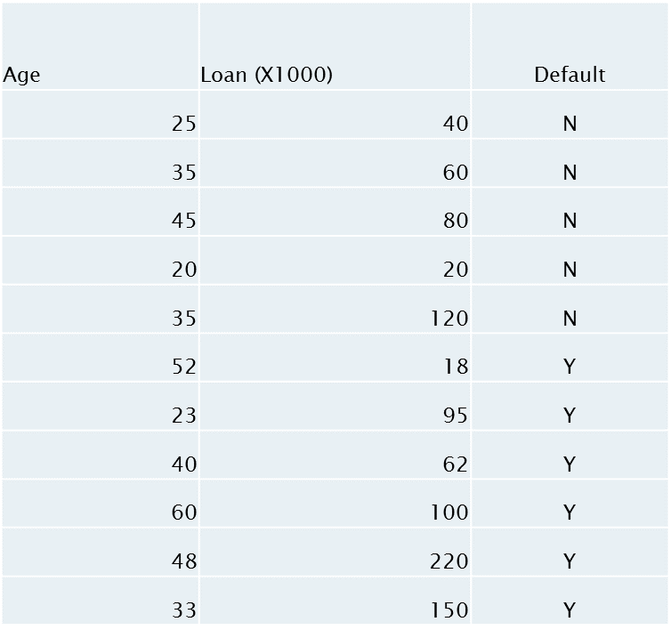
age<-c(25,35,45,20,35,52,23,40,60,48,33)
loan<-c(40,60,80,20,120,18,95,62,100,220,150)
default<-c("N","N","N","N","Y","Y","Y","Y","Y","Y","Y")
K-Means Algorithm
So far we have discussed 2 supervised learning algorithms: one for classification (K-NN) and another regression (Linear regression). Supervised means that we know the results for some datasets, we learn from it and apply the knowledge to predict or label the query data. In the classification case, output variable is a "class" or category, nd in the regression case, it is a value. Here are some details about K-means:- K-means is unsupervised: no prior knowledge of the “right answer”
- Goal of the algorithm Is to determine the definition of the right answer by finding clusters of data
- Kind of data: satisfaction survey data, survey data, medical data, SAT scores Assume data {age, gender, income, state, household, size}, your goal is to segment the users.
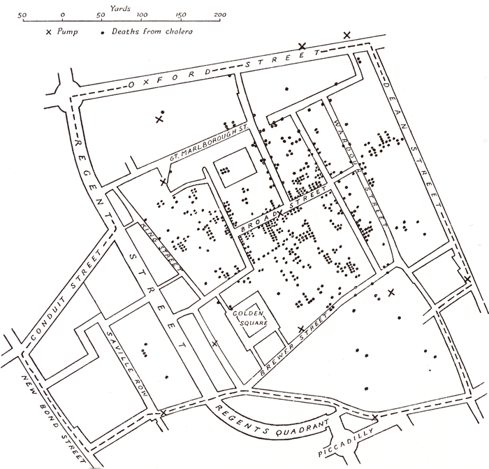
- Lets understand kmeans using an example. Also read about “birth of statistics” in John Snow’s classic study of Cholera epidemic in London 1854: “cluster” around Broadstreet pump: http://www.ph.ucla.edu/epi/snow.html
K-means Algorithm
- Initially pick k centroids
- Assign each data point to the closest centroid
- After allocating all the data points, recomputed the centroids
- If there is no change or an acceptable small change, clustering is complete Else continue step 2 with the new centroids.
- Output: K clusters Also possible that the data may not converge. In that case, stop after certain number of iterations.
- Evalaution metric: between_ss/total_ss, range 0-1, for good tight clustering, this metric is as close to 1 as possible.
23 25 24 23 21 31 32 30 31 30 37 35 38 37 39 42 43 45 43 45
Lets cluster it for K = 3
See Demo code here