Table of contents
- Mobile Robot Mapping
- Motivation for Mapping
- Background to Mapping
- Conventional Notation
- Mapping with known poses
- Scan matching
- Loop Closure
- Iterative Closest Point, ICP
- ICP Algorithm
- Point-to-point ICP derivation
- Alternative ICP methods
- Mapping in 3D
- Map representations
- Occupancy grid update derivation
- Odometry/Dead reckoning
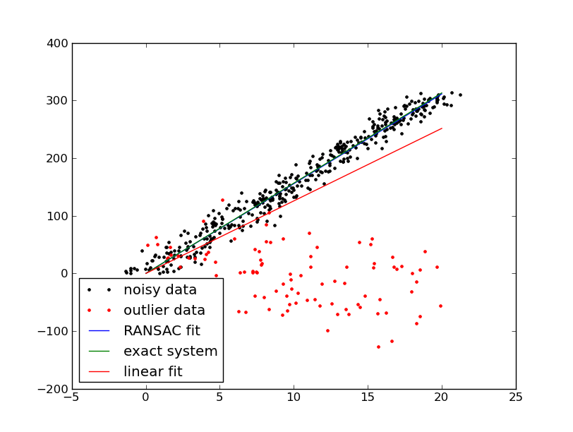
- RANdom SAmple Consensus, RANSAC
- RANSAC pseudocode
- RANSAC Illustration
- Feature extraction
- Current research
- Good Related Courses
- References
Motivation for Mapping
Insufficient GPS accuracy
No GPS indoors
- Prerequisite for many mobile robot tasks
- Path planning
Sometimes robots effective without it e.g. iRobot Roomba series
Maps for humans
Background to Mapping
- Aspects to mapping
- Localisation
- Mapping
- Simultaneous Localisation and Mapping SLAM
- Type of maps
- Geometric mapping
- Topological mapping
Conventional Notation
- Pose - position + orientation, X
- Map, M
- Sensor data, Z
- Sensor model is \(p(Z|M, X)\)
Canonical form of map building, map given set of sensor measurements and corresponding poses
Recast by Bayes' theorem
Scan matching
Iterative Closest Point, ICP
RANSAC
- Cumulative errors like odometry
- Scan to scan
- Scan to map
Address these with loop closure
Further details see Scan-matching
Typical convergence path http://www.youtube.com/watch?v=LlevpwUrWkE
Loop Closure
- Two main elements
- Place recognition
- Pose graph error distribution
Loop closure dramatically improves quality of large scale maps
A Heuristic Loop Closing Technique for Large-Scale 6D SLAM by J. Sprickerhof, A. Nüchter, K. Lingemann, and J. Hertzberg
Iterative Closest Point, ICP
- Purpose to align points
- originally devised for aligning 3D scan point clouds scanners
Original paper [besl1992]
- Implementations
- PCL point cloud library
- Meshlab
- MRPT Mobile robotics programming toolkit
ICP Algorithm
For two sets of points P and Q.
- while E > threshold
- Establish correspondences e.g. by nearest neighbour
- Estimate transformation parameters using a mean square cost function.
- Transform points using the estimated parameters.
- Calculate E
Point-to-point ICP derivation
For a rotation about the x-axis
Given the rotation matrices around the various axes.
The full rotation matrix for small angles \(\alpha, \beta, \gamma\) about the \(x, y, z\) axes is therefore
The rotation matrix,
The translation vector
The error function
To minimise E equate partial derivatives to zero.
Factor out the coefficients of the DOFs appropriately so it can be represented in linear form for solving.
Results in a covariance like matrix and linear matrix equation
- A is symmetric so Cholesky decomposition is recommended
Alternative ICP methods
- Derivation of point-to-plane minimization by Szymon Rusinkiewicz ICP derivation
- Generalized ICP by A. Segal, D. Haehnel and S. Thrun
Mapping in 3D
Dense Occupancy grids do not scale well to 3D
- Alternatives
- Point clouds
- Store Occupied Voxels only
Octrees
Map representations
- Geometric Maps
- Occupancy Grids
- Feature/landmark maps
- Occupancy Grids
- Probability or measure that a cell is occupied
- Good for path planning
- Update mechanism
- log likelihood update
Occupancy grid update derivation
Canonical form of map building, map given set of sensor measurements and corresponding poses
Under first-order Markov assumption
Applying these assumptions gives rise to
Finally, this produces
which only holds if the environment is time invariant.
For a particular map cell, m, and laser return cell, l
The log odds approach to probabilities simplifies the update step enhances the expressive power of the map, which often contains probabilities close to either 1 or 0
The odds of an event A
and conversely probabilities can be calculated from the odds as
Thus the map update can be expressed as
Therefore in terms of log odds
Odometry/Dead reckoning
Normally insufficient on its own for map building
Good for providing high speed initial guess
- Sources of odometry
- wheel encoders
- IMU, gyroscopes
- Combination of IMU and wheel encoders can be good
RANdom SAmple Consensus, RANSAC
- Overview
- Iterative method for model parameter estimation
- Good generic goto algorithm
- In real world data outliers are usually possible
- Advantages
- Robust to outliers
- Simple to implement and effective
- Anytime algorithm
- Disadvantages
- Can take a long time
- Requires some parameters
- Number of elements required for a good fit
- Inlier/Outlier distance threshold
- Number of iterations
RANSAC pseudocode
while iterations < k
    maybe_inliers := n randomly selected values from data
    maybe_model := model parameters fitted to maybe_inliers
    consensus_set := maybe_inliers

    for every point in data not in maybe_inliers
        if point fits maybe_model with an error smaller than t
            add point to consensus_set

    if the number of elements in consensus_set is > d
        (this implies that we may have found a good model,
        now test how good it is)
        this_model := model parameters fitted to all points in consensus_set
        this_error := a measure of how well this_model fits these points
        if this_error < best_error
            (we have found a model which is better than any of the previous ones,
            keep it until a better one is found)
            best_model := this_model
            best_consensus_set := consensus_set
            best_error := this_error

    increment iterations
Feature extraction
- Many SLAM algorithms rely on landmarks
- How do we get these landmarks?
Various levels of feature extraction
- 3D occupancy grid --- Extension of 2D occupancy grids
- Occupied voxel list --- Occupied voxels only
- Edge voxel map --- Non-planar voxels
- Feature map --- List of point features and their covariances
References
Simultaneous Localisation and Mapping (SLAM): Part I The Essential Algorithms Hugh Durrant-Whyte, Fellow, IEEE, and Tim Bailey
| [besl1992] | A method for registration of 3D shapes |


