Systems and Control
- Reading
- Maki, Nordlund and Eklundh, Attentional scene segmentation: Integrating depth and motion from phase, Computer Vision and Image Understanding v 78 (2000), 351-373.
We conclude our study of active and animate vision with a look at how the various skills (motion, OR, etc.) can be pulled together into a goal-directed system, and how the behavior of that system can be controlled.
An important element of any active vision system is gaze control, that is, control of the field of view by manipulation of the optical axis and other extrinsic camera model parameters, and control of the regions of interest (ROI) within the current field of view which require further processing.
Even without moving your eyes, you can change the locus of attention from one region of the field of view to another. This is called attentional gaze control, and is the subject of the Maki paper. He likens this to cognitively "shining a spotlight" on a selected portion of the retinal image without any change in the camera model.
For artificial active vision systems, it is essential to be able to select those ROI's that need further analysis effectively and quickly. The identification of these ROI's is attentional scene segmentation, i.e. segmenting out interesting parts of the scene for further processing.
The approach to attentional scene segmentation proposed in this paper is a cue integration approach. Three visual cues which together define the most important ROI's for additional consideration and processing are computed, masks defining their locations and extent within the field of view determined, and the their intersection determined. These regions correspond to the ROI's for "attention."
Why do we need attentional segmentation? Both in natural and in computer vision, in general there are two kinds of processing of raw image brightness data: preattentive and attentive processing.
- Preattentive processing
- preeprocessing which occurs automatically and uniformly over the field of view independent of space or time.
- Attentive processing
- processing of ROI's determined by the vision system's attention control mechanism to merit additional "attention," i.e. analysis.
Eg: There is a parked car 100 meters ahead in the periphery of our field of view as we are walking in a parking lot. If we are simply doing obstacle avoidance, a stationary distant car does not trigger our attention control mechanism, we need not attend to it. But if we are trying to find our car in the lot, we will need to process that information further, probably by foveating to it.
Like everything else in an active vision system, the attentive control decision process is both task and embodiment dependent.
Often the result of attentive scene segmentation is to identify ROI's we need to foveate to. But another use is to trigger reactive (stimulus-response) rather than cognitive (stimulus-analysis-planning-response) behavior.
Eg: we are walking through the woods and are about to collide with an overhanging branch which suddenly appears in our FOV. We attentively segment out the branch and react to its radial motion and location, ducking away from it without foveating to it if the threat is immediate. Note: recall the threat metric
\(1/t_c = (dr_i/dt)/r_i \)
and that foveation requires at least 100 ms for the human eye.
Preattentive processing produces, at each time t and at each point (u,v) in the image space, a vector of values for the preattentive image parameters at that point. Each component can be considered a preattentive cue for attentive segmentation. Maki et al select 3:
- image flow
- stereo disparity
- motion detection
There are many other preattentive cues that might have been selected: edges, colors, color gradients,region sizes, etc. They pick these because they believe the most important things to attend to in in general, i.e. preattentively, for further processing are nearby objects in motion relative to the viewer.

Attentional integration of selected preattentional cues
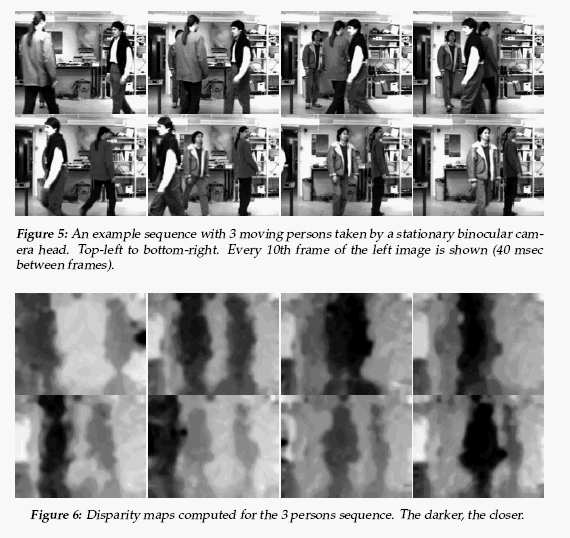
Stereo disparity is the difference between where a given point in world coordinates shows up on the two image planes. From stereo disparity we can determine relative depth. Attentional attractiveness in this cue is low relative depth . Maki et al compute a dense stereo disparity map by using a phase based method. There are other ways to do this, including the sparse feature-based and dense correlation-based methods we discussed earlier.
Optical flow may be used to determine motion in the plane perpendicular to the optical axis. Under orthographic projection, optical flow is completely insensitive to depth motion, and for distant objects, perspective projection and orthographic projection are very similar.
Maki et al choose to measure only the 1-D horizontal component of flow in the plane perpendicular to the optical axis because they can reuse the 1-D depth discovering disparity algorithm to do this.
Motion detection is employed to segment regions where motion is occurring, and together with optical flow then used to determine the constancy of that motion in image regions for purposes of multi-object segmentation.
Stereo disparity cue
Stereo disparity measures relative depth. Image points of equal disparity are at the same depth.

We see that depth is not a function of rt, just of stereo baseline \(2r_0\) and disparity. So for a given intrinsic stereo camera model, disparity measures relative depth.
The algorithm for determining the disparity at image point (x,y) used in Maki et al uses phase difference at a known frequency to determine spatial difference.
- Using a Fourier wavelet-like kernel, compute the magnitude and phase V(x) of the horizontal frequency component at the image location x. Repeat for left and right images.
- Disparity, \(D(x) = ((\arg(V_l(x))-\arg(V_r(x)))/2 \pi)*T\)
- \(T = 2\pi/ \omega\), where \(\omega \approx d/dx_1 (\arg(V(x))\)
For details see the earlier paper by Maki et al
- Phase-Based Disparity Estimation in Binocular Tracking, A. Maki, T. Uhlin, J-O Eklundh
Optical flow cue
Suppose we determine \(V_{t_1}(x)\) and \(V_{t_2}(x)\), where \(t_1\) and \(t_2\) are successive image acquisition times, \(V_{t_1}(x)\) and \(V_{t_2}(x)\) are taken by the same camera. Then the "disparity" measured as above corresponds to image flow in the horizontal direction. In this case T corresponds to a temporal rather than a spatial period as before.
We cover the same optical flow approach in 05.
A problem with this common method for disparity and optical flow is that it may give unreliable point estimates of these two cues.
They define a confidence parameter (certainty map) C(x) which is the product of the correlation coefficient between the two V's and their combined strength (geometric mean magnitude).
The idea is that x's where the V's are similar and are strong are reliable for using their associated cues to determine attentional masks.
Having now mapped both disparity and optical flow separately over the field of view, we need to segment out regions that are identified by these cues as requiring further processing. This of course is task dependent. Maki et al define two generic task modes, pursuit mode and saccade mode. Pursuit mode includes visual servoing, shape from motion, and docking. Saccade mode includes visual search, object detection, object recognition.
Pursuit mode
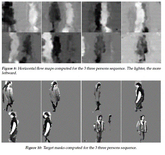
This is also called tracking mode, where the task is to continue to attend to a moving target that has already been identified. The procedure to create the disparity mask \(T_d(k)\) and image flow mask \(T_f(k)\) at time k is the same:
- Predict the change P(k) from k-1 to k in the disparity (flow) target value based on a simple linear update of P(k-1).
- Let the selected disparity (flow) value at k be the sum of that at k-1 plus P(k).
- Find the nearest histogram peak to the selected value and define that histogram mode as target values. Note: the histograms are confidence-weighted.
Finally, the target mask \(T_p(k)\) is defined as the intersection of the disparity mask \(T_d(k)\) and image flow mask \(T_f(k)\). This guarantees that the target we will attend to is both in the depth range we predict and has the horizontal motion we predict.
Saccade mode
Here the task is to identify the region containing the most important object that you are not currently attending to. The authors admit that importance is definitely task dependent, but stick with their assumption that close objects in motion are the most important ones.
- Eliminate the current target mask from the images and compute confidence-weighted disparity histograms.
- Back-project the high disparity (low depth) peaks, again eliminating current target mask locations.
- Intersect with motion mask. Finally, the least-depth region in motion is the output saccade mode target mask.
Choosing between pursuit and saccade at time k
At each time k, we may choose to continue pursuit of the current target in the pursuit map \(T_p(k)\) (if there is one), or saccade to the new one in the saccade map \(T_s(k)\).
There are many criteria that could be employed to preference between these alternatives. Some take their input directly from the two maps, others reach back into the data used to compute them. For instance:
- Pursuit completion: pursue until a task-completion condition is met. For instance, object recognition or interception.
- Vigilant pursuit: pursue for a fixed period of time, then saccade, then return to pursuit.
- Surveillance: saccade until all objects with certain characteristics within a set depth sphere have been detected.
Consistent with their depth-motion framework, Maki et al suggest two different pursuit-saccade decision criteria: Depth-based: pursue until the saccade map object is closer than the pursuit map object.
Duration-based: pursue for a fixed length of time. Clearly, neither of these is sufficient. The depth-based criterion is not task or embodiment dependent. We may let an important target "get away" by saccading to a closer object that is for instance moving away from us. And bad things can happen to us during the duration-based fixed time that we are not alert to obstacles and threats.
Example from their paper:
As a final note, lets measure the Maki et al attentive gaze control approach against the active vision and animate vision paradigms.
-
Active vision: Compute what you need as you need it
- Representations and algorithms minimal for task.
- Vision is not recovery.
- Vision is active, i.e. current camera model selected in light of current state and goals.
- Vision is embodied and goal-directed.
-
Animate vision: Anthropomorphic features emphasized
- Binocularity: NA
- Foveal (multiresolution) focal plane geometry
- Gaze control, both between and within eye movements
- Use fixation frames and indexical reference