Date	Topic and Chapter	Classnotes	Handouts
1/29	Introduction to Data-Intensive Computing: Ch.1		classnotes
1/31	The Data Science Road Map: Ch 2	DS Roadmap	JupyterRStudio Handout
2/5	Lab 1 Discussion	Lab1	Lab1 Files
2/7	Exploratory Data Analysis (EDA)	Intro to R	Demo Data
2/12,14	Statistical Modeling and ML Algorithms	Models and Algorithms in R	Demo Description
2/14	Lets Review EDA & Algorithms for EDA	Models and Algorithms in R	Demo links inline
2/19	Data Infrastructure	Introduction to MapReduce	InfraStructure I
2/26	Big Data Infrastructure	Hadoop, Yarn and Beyond	InfraStructure II
2/28	Big Data Algorithms	MapReduce	Algorithms
3/5	Design MR Solutions	MapReduceCombiner	Algorithms
3/12	Demo and discussion of MR.HDFS	Download Hadoop, Demo Uspres speeches	MapReduce: How to code?
3/29	Review for Exam; Clarification on Lab2	MR.Hadoop; Data Analysis Algorithms	Exam Review
4/2	Word Co-occurrence	MR.Hadoop; Data Analysis Algorithms	WordCO
4/4	Graph Algorithms	MR.Hadoop; Data Analysis Algorithms	Graph Alg
4/9	Apache Spark	Notes	Apache Spark
4/18	Naive Bayes	Notes	Bayesian Classification
4/23	Logistic Regression & ML Overview	Notes	ML and Logit Classification
4/25	Working on spark	Lab3: How to get started?	Working on Spark
4/25	Evaluating the Classifiers	Applies to Lab3 and Final Exam	Evaluation Metrics
5/2	Take inventory of what you learned	Final Exam Topics	Course Review
5/7	Final Review	Final Exam Topics	Review for the Final Exam

1. "Hmm..What is Data-intensive Computing?"

January 29 by Bina

The phrase was initially coined by National Science Foundation (NSF). This particular definition sets a very nice context for our course.

Before we go further let's set the context. We are living in a golden era in computing.

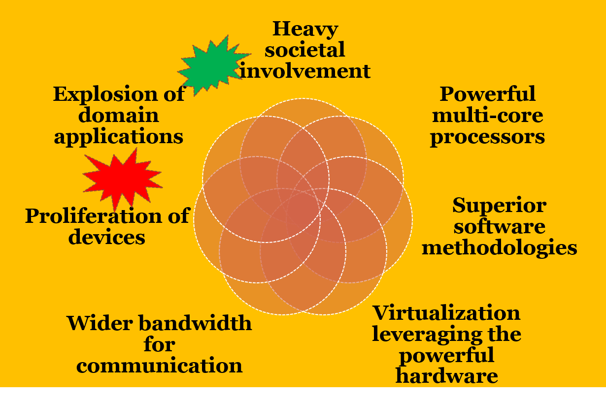
2. Given this context, how can you characterize data..big data?

Volume, velocity, variety, veracity (uncertainty) (Gartner, IBM) as illustarted here

3. How are we addressing the increased complexity in data?

Tremendous advances have taken place in statistical methods and tools, machine learning and data mining approaches, and internet based dissemination tools for analysis and visualization. Many tools are open source and freely available for anybody to use.
More importantly, newer storage models, processing models, big data analytics and cloud infrastructures have emerged.

4. Okay. Can you give us some examples of data-intensive applications?

• Search engines
• Recommendation systems: CineMatch of Netflix Inc. movie recommendations
  Amazon.com: book/product recommendations
• Biological systems: high throughput sequences (HTS)
  Analysis: disease-gene match
  Query/search for gene sequences
• Space exploration
• Financial analysis

5. What about the scale of data?

Intelligence is a set of discoveries made by federating/processing information collected from diverse sources. Information is a cleansed form of raw data.

For statistically significant information we need reasonable amount of data.

For gathering good intelligence we need large amount of information.

As pointed out by Jim Grey in the Fourth Paradigm book enormous amount of data is generated by the millions of experiments and applications. Thus intelligence applications are invariably data-heavy, data-driven and data-intensive.
Lets discuss algorithm vs data. "More data beats better algorithms".

6. How about data applications? Characteristics of intelligent applications

Google search: How is different from regular search in existence before it? It took advantage of the fact the hyperlinks within web pages form an underlying structure that can be mined to determine the importance of various pages.
Restaurant and Menu suggestions: instead of “Where would you like to go?” “Would you like to go to CityGrille”? Learning capacity from previous data of habits, profiles, and other information gathered over time.
Collaborative and interconnected world inference capable: facebook friend suggestion Large scale data requiring indexing
…Do you know amazon is going to ship things before you order?

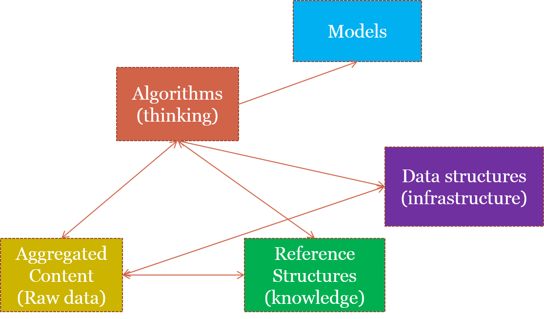
7. Data-intensive Computing Model (From Lin & Dyer)

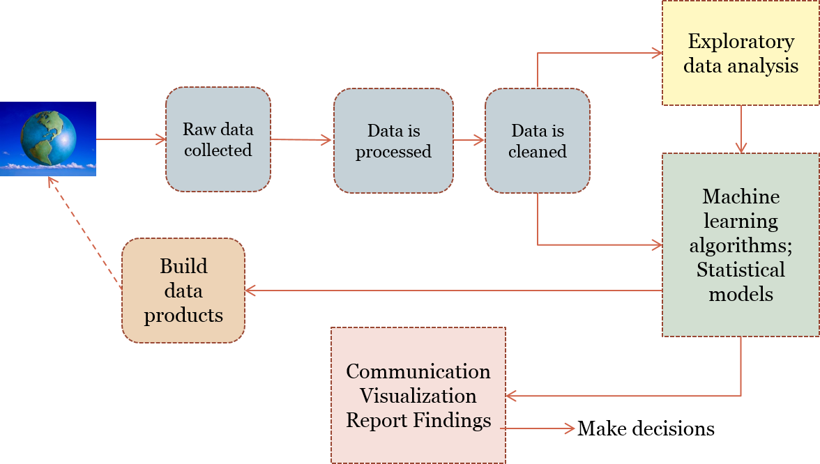
8. Data Science Process I(Adapted from Doing Data Science)

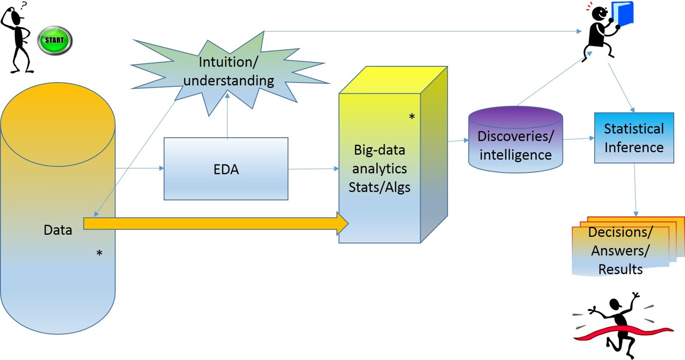
9. Data Science Process II

10. How do we plan to do it?

Small units of learning: conceptual and applied, reinforced by the lab assignment. In the recommeded text book, the author Field Cady organizes the it into three parts:

1. The core: Skills that are absolutely indispensible at any level of data science.
2. The additional core: Skills you need to know, but may not use it all the time.
3. Stuff good to know: Expansion of the core topics and theoretical background.

EDA and Algorithms for Data Processing

February 19 by Bina

We reviewLinear Regression.

Problem 1: Consider the data

S = {(x,y)= (1,25), (10,250), (100,2500), (200,5000)}

What next? What is value for X = 40?
We observe that

• There is a linear pattern.
• Coefficient relating x and y is 25
• Seems deterministic
• and y = 25*x is the relationship, an obvious linear pattern.

Linear model is defined by the functional form:
y = β0 + β1*x

Lets work on 2 demos:

A simple analysis of "cars" data already available in R environment Another demo to understand the evaluation metric for an "lm" . Goal is to visualize and understand lm and its statistics.
1. The second demo is on synthetic data to understand the importance of the evalaution metrics and also to understand "overfitting"

For each demo we are interested in:

1. Cleaning and getting a data frame
2. Plot the data points
3. Visually assess the data plot
4. Model using "lm"
5. "lm" by default seeks to find a trend line that minimizes the sum of squares of the vertical distances between the approximated or predicted and observed y's.
6. We want to learn both the "trend" and the "variance"
7. Evaluate the measure of goodness of our model in R-squared and p: R-square measures the the proportion of variance. p-value assesses the significance of the result. We discuss both these measures: we want R-sqaured to high (0.0-1.0 range) and p to be low or <0.05. R-squared is 1-(total predicted error-squared/total mean error squared)

See Demo code here

Linear Regression Evaluation Metric

1. Goodness of fit:
R2 range is 0-1. For a good fit we would like R2 to be as close to 1 as possible. R2 = 1 means every point is on the linear regression line!
The second term represents the "unexplained variance" in the fit. You want this to be as low as possible.
2. Quality of data p: Low p means Null hypothesis (H0) has been rejected. We would like p <0.05 for high significance of prediction.

K-NN Algorithm

• K-nearest neighbor
• Supervised machine learning
• You know the “right answers” or at least data that is “labeled”: training set
• Set of objects have been classified or labeled (training set)
• Another set of objects are yet to be labeled or classified (test set)
• Your goal is to automate the processes of labeling the test set.
• Intuition behind K-NN is to consider K-closest items for similarity --- similarity defined by their attributes, look at the existing label and assign the test object the label.

Intuition

See Demo code here

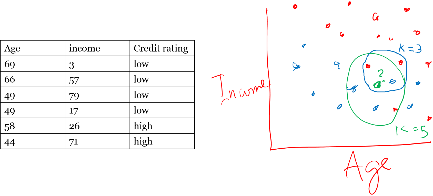
Lets Review K-NN

General idea is that a data point will similar to its neighbors. So classify it or label it accordingly. Which neighbor(s), how many neighbors?
Here is an overview of the process:

1. Decide on your similarity or dsitance metric
2. Split the original set into training and test set
3. Pick an evalaution metric: Misclassification rate is a good one
4. Run K-NN few times, changing K and checking the evaluation metric
5. Once best K is chosen, create the test cases and predict the labels for these

Euclidian distance is a good similarity metric. Scale of the features (or variable) should be almost same for this to work well.
Manhattan distance (X+Y) is another, data need not be normalized.
Hamming, Cosine distance are other.
Lets try it out with a sample data set:

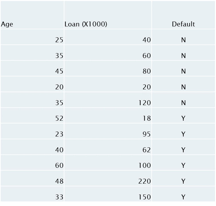
age<-c(25,35,45,20,35,52,23,40,60,48,33)
loan<-c(40,60,80,20,120,18,95,62,100,220,150)
default<-c("N","N","N","N","Y","Y","Y","Y","Y","Y","Y")

Lets simulate it on paper and compare with R. Rcode is here .

K-NN Issues

• How many nearest neighbors? In other words what is the value of k
  Small K: you overfit
  Large K : you may underfit
  Or base it on some evaluation measure for k choose one that results in least % error for the training data (we will do this in today's demo)
• Implications of small k and large k
• How do define similarity or closeness?
  Euclidian distance
  Manhattan distance
  Cosine similarity etc.
• Error rate or misclassification (k can be chosen to lower this)
• Curse of dimensionality

K-Means Algorithm

So far we have discussed algorithms for EDA: one for classification (K-NN) and another regression (Linear regression). For these algorithms we know the results for some datasets, we learn from it and apply the knowledge to fit a model, predict or label the query data. In the classification case, output variable is a "class" or category, dnd in the regression case, it is a value. Now lets review Kmeans. Here are some details about K-means:

• K-means is unsupervised: no prior knowledge of the “right answer”
• Goal of the algorithm Is to determine the definition of the right answer by finding clusters of data
• Kind of data: satisfaction survey data, survey data, medical data, SAT scores Assume data {age, gender, income, state, household, size}, your goal is to segment the users.
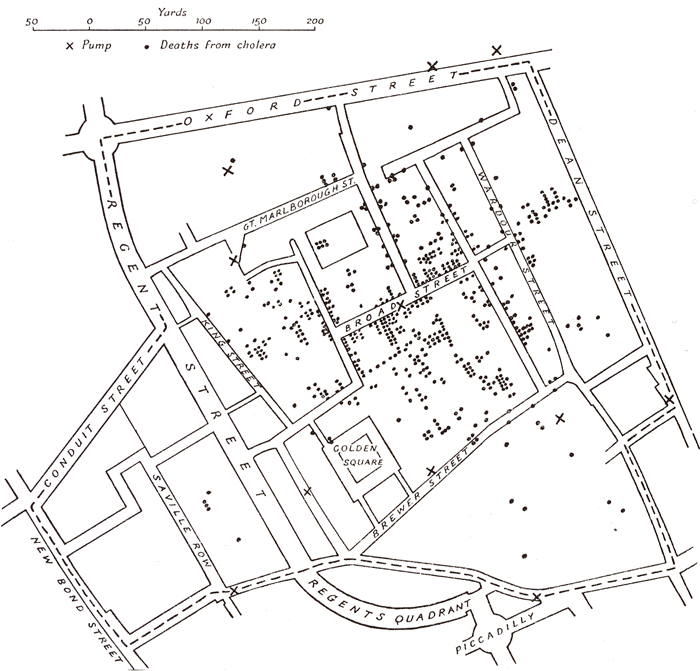
• Lets understand kmeans using an example. Also read about “birth of statistics” in John Snow’s classic study of Cholera epidemic in London 1854: “cluster” around Broadstreet pump: http://www.ph.ucla.edu/epi/snow.html

K-means Algorithm

1. Initially pick k centroids
2. Assign each data point to the closest centroid
3. After allocating all the data points, recomputed the centroids
4. If there is no change or an acceptable small change, clustering is complete Else continue step 2 with the new centroids.
5. Output: K clusters Also possible that the data may not converge. In that case, stop after certain number of iterations.
6. Evalaution metric: between_ss/total_ss, range 0-1, for good tight clustering, this metric is as close to 1 as possible.

23 25 24 23 21 31 32 30 31 30 37 35 38 37 39 42 43 45 43 45
Lets cluster it for K = 3
See Demo code here

Data Infrastructure

February 19 by Bina

Introduction

In the 1990's during the early days of the Internet, the access mode for home computing was through a humongous modem that made this characteristic noise. People had one of the two or three service providers: Prodigy, or Compuserve and probably the web and the search was the only application. Even that was slow. The "web page" was not fancy since most people had only line-based terminals for accessing the Internet. One of the popular browsers was called "Mosaic". When you query for the something it took such a long time that you can clean up your room by the time the query-results arrived.

In late 1990's Larry Page and Sergei Brin (Standford graduate) students worked on the idea considering the web as a large graph and ranking the nodes of this connected web. This became the core idea for their thesis and the company they founded, Google. Google that has since become the byword for "search". The core idea is an algorithm called "Pagerank". This is well explained in a paper [1] written about this thesis.

Until Google came about the focus was on improving the algorithms and the data infrastructure was secondary. There were questions about the storage use for supporting this mammoth network of pages and their content that are being searched. In 2004 two engineers from Google presented an overview paper [2] of the Google File System (GFS) and a novel parallel processing algorithm "MapReduce". A newer version of the paper is available at [3] .

Of course, Google did not release the code as open source. Doug Cutting an independent programmer who was living in Washington State reverse engineered the GFS and named it after the yellow toy elephant that belonged to his daughter. Yahoo hired him and made Hadoop open source.

In 2008 Yahoo, National Science Foundation and Computing Community Consortium gathered together educators, industries, and other important stakeholders for the inaugural Hadoop Summit. Look at the list of attendees here I learned Hadoop from Doug Cutting. It is imperative that we study Hadoop and MapReduce together to learn their collective contribution.

Let us understand the foundation of the Big Data Infrastructure that has become integral part of most computing environments. We will approach this study by processing unstructured data as discussed in text [4] .

References

1. K. Bryan and T. Leise. The $25,000,000,000 Linear Algebra Behind Google. here.
2. Dean, J. and Ghemawat, S. 2004. MapReduce: Simplified data processing on large clusters. In Proceedings of Operating Systems Design and Implementation (OSDI). San Francisco, CA. 137-150. MR, last viewed 2017.
3. Newer version in ACM of the above paper here.
4. J. Lin and C. Dyer. Data-Intensive Text Processing with MapReduce, Synthesis Lectures on Human Language Technologies, 2010, Vol. 3, No. 1, Pages 1-177, (doi: 10.2200/S00274ED1V01Y201006HLT007). Morgan & Claypool Publishers. An online version of this text is also available through UB Libraries since UB subscribes to Morgan and Claypool Publishers. Online version available here